The dark energy equation of state (EOS) is defined as
w(a) ≡ p(a) / ρ(a) , |
w(a) = w0 + wa(1-a) . |
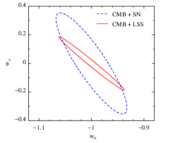
We want to evaluate future experiments based on the area enclosed by the 68.3% confidence level contour for the two parameters w0 and wa. In this example we compare CMB + SN against CMB + LSS.
Open file headfiles/options.h. Find the line #define DARK_ENERGY_MODEL COSMOLOGICAL_CONSTANT. Change it to #define DARK_ENERGY_MODEL W0WA_MODEL. Save the file. Recompile the package
./clear.sh ./compile.sh |
You need a new inifile and fidfile to produce the mock data. Make a copy of forecast/lcdm.ini and forecast/lcdm.fid.
cd forecast/ cp lcdm.ini w0wa.ini cp lcdm.fid w0wa.fid |
Open the file w0wa.ini. Set
fidfile = w0wa.fid
action = -1
simulate_CMB = T
simulate_LSS = T
simulate_SN = T
Now we need to set the fiducial parameters. Let us now have a closer look at the indices of the parameters. The parameters are separated into 4 blocks. The first block contains "basic parameters". The second block contains "dark energy parameters". The third block contains "primordial power spectra parameters". The last block contains the "nuisance parameters" that are not directly related to cosmology. The length of the four blocks are defined in headfiles/options.h. Find the lines
#define NUM_BASIC_PARAMS 6
#define NUM_DE_PARAMS 4
#define NUM_POWER_PARAMS 5
That means 6 basic parameters, 4 dark energy parameters, and 5 primordial power spectra parameters. The number of nuisance parameters is the sum of the number of CMB, LSS, SN, WL...(some options are for future extensions) nuisance parameters. We will not use any nuisance parameters in this example (LSS and SN nuisance parameters are all marginalized analytically in the likelihood). Note that each block has a minimal length (4, 3, 5, 5 respectively). We will keep the default setting with 3 CMB nuisance parameters and 2 SN nuisance parameters to make the code compile. For the same reason we will keep 4 dark energy parameters, although we only need 2.
If you have set USE_COSMOMC_THETA = YES in /headfiles/options.h, the first four basic parameters are Ωbh2(physical density of baryons today), Ωch2 (physical density of cold dark matter today), θ (100 times the angle that sound horizon extends on the last scattering surface), and τre (reionization optical depth).
If you have set USE_COSMOMC_THETA = NO, the first four basic parameters are Ωb (energy fraction of baryon), Ωm (energy fraction of baryon + cold dark matter), h (reduced Hubble parameter), and τre.
The 5th and 6th parameters are not used. They are reserved for future extensions to open/closed universe and massive neutrinos.
Since we are using 6 basic parameters, the indices of the 4 dark energy parameters are 7, 8, 9, 10. How do we know which two are w0 and wa ? The index of each individual parameter is defined in headfiles/define_MCMC_params.h. Open this file and find the following two lines
#define INDEX_W0 (INDEX_DE + 1)
#define INDEX_WA (INDEX_DE + 2)
Since there are totally 6 basic parameters and 4 dark energy parameters, the indices of the five primordial power spectra parameters are 11, 12, 13, 14, 15.
The physical meaning of these parameters depends on what model of primordial power spectra you are using. By looking at headfiles/options.h again, you figure out that we are using
PRIMORDIAL_POWER = NSNRUN_MODEL
From the comments above this entry, you learn that the 5 parameters are ns (the spectral index of the primordial scalar power spectrum), nt (the spectral index of the primordial tensor power spectrum), nrun (the running of the spectral index of the primordial scalar power spectrum, in some literature it is called αs), ln(1010As) (the logarithm of the amplitude of the primordial power spectrum at a pivot k = 0.05 Mpc-1), and r (the tensor to scalar ratio at the same pivot).
Knowing what the 20 parameters are, we now open and edit the file forecast/w0wa.fid. Change the root data/LCDM to
data/W0WA
Change the second non-comment line to the fiducial parameters. For example , you choose a model with Ωbh2 = 0.022, Ωch2 = 0.1128, θ = 1.4617 , τre = 0.09, w0 = -1, wa = 0 , ns = 0.968, nt = 0, nrun = 0 , ln(1010As) = 3.027, and r = 0.128. The second non-comment line then should be:
0.022 0.1128 1.04617 0.09 0 0 -1 0 0 0 0.968 0 0 3.027 0.128 0 0 0 0 0
Choose proper lower-bounds, upper bounds and step sizes of the parameters. We will fix nt = 0 and nrun = 0. The list of varying parameters is Ωbh2, Ωch2, θ, τre , w0 , wa , ns , ln(1010As), and r. Totally 9 varying parameters.
Example of the lower-bounds:
0.01 0.05 0.5 0.02 0 0 -3 -3 0 0 0.5 0 0 2.4 0 0 0 0 0 0
Example of the upper-bounds:
0.1 0.5 2. 0.14 0 0 1 3 0 0 1.5 0 0 4. 1 0 0 0 0 0
Example of the step sizes
0.0002 0.001 0.0003 0.001 0 0 0.01 0.05 0 0 0.002 0 0 0.002 0.02 0 0 0 0 0
OKay! We finally went through the fidfile hacking. Save the file w0wa.fid. Run
./cosm w0wa.ini |
Mock data are produced. Check out the files forecast/data/W0WA_CMB.dat etc.
We first calculate the covariance matrix for CMB + LSS. Open the inifile w0wa.ini. Set
action = 2
output = chains/w0wa_CMBLSS
simulate_CMB = T
simulate_LSS = T
simulate_SN = F
Run
./cosm w0wa.ini |
Do the same for CMB + SN. Set
output = chains/w0wa_CMBSN
simulate_CMB = T
simulate_LSS = F
simulate_SN = T
Run
./cosm w0wa.ini |
Open the file forecast/chains/w0wa_CMBLSS_fisher.info and forecast/chains/w0wa_CMBSN_fisher.info. You find the standard deviations of w0 (index = 7) and wa (index = 8). However, that does not tell you much, because w0 and wa are strongly correlated with each other. What matters is the figure of merit (FOM), which is inversely proportional to the determinant of their covariance matrix.
The better way to present the result is to visualize the constraints in a figure. For which we need to...(guess?) Yes, go to the directory postprocess.
cd ../postprocess |
Open the file pfparams.ini. This inifile defines how you want to make the figure (file name, width, height, legends etc.). Set
output_file = w0wa.eps
covmat_file_1 = ../forecast/chains/w0wa_CMBSN_fisher.info
covmat_file_2 = ../forecast/chains/w0wa_CMBLSS_fisher.info
Run
./pf pfparams.ini |
You get a figure w0wa.eps. It looks like this:
| model | Setting in headfiles/options.h | parameter list in the 2nd parameter block |
|---|---|---|
| Cosmological Constant (w=-1) | #define DARK_ENERGY_MODEL COSMOLOGICAL_CONSTANT | (unused, unused, unused, unused) |
| w = w0 | #define DARK_ENERGY_MODEL CONSTANT_W_MODEL | (w0, unused, unused, unused) |
| w = w0 + wa(1 - a) | #define DARK_ENERGY_MODEL W0WA_MODEL | (w0, wa, unused, unused) |
| w = w(Ωm0; εs; ε∞; ζs; a)
General parametrization of minimally coupled quintessence. See arxiv:1007.5297 | #define DARK_ENERGY_MODEL QCDM_MODEL | (εs, ε∞, ζs, unused) |
Dark energy perturbations are treated as perfect fluid with sound speed cs2 = 1 . When w crosses the phantom line w = -1, extra degree of freedom is required for fully self-consistent treatment. Since there is no preferred model, I simply freezes the dark energy perturbations when the crossing happens. See also Fang, Hu and Lewis 2008 where a better treatment is given.
The primordial scalar power spectrum and primordial tensor power spectrum of the metric fluctuations are parameterized as
Δs2 = As (k / k*)ns - 1 + 1⁄2 nrun ln (k/k*) , Δt2 = At ( k / k* )nt , r ≡ At / As . |
This model is called "NSNRUN_MODEL" in CosmoLib. Sometimes people use different pivot k for scalar and tensor. Since the spectral index of tensor spectrum will not be measurable in the near future, using different pivots does not make a significant difference. We will not bother to do that. The pivot k* is always taken to be 0.05Mpc-1.
In headfiles/options.h you can find the line
#define PRIMORDIAL_POWER_MODEL NSNRUN_MODEL
#define NUM_POWER_PARAMS 5
These two lines define the standard case with five parameters in the 3rd parameter block: ns, nt, nrun, ln(1010As), and r.
There are other options, however. One example is the axion monodromy model. To very good approximations, the primordial power spectra can be parameterized as
Δs2 = As (k / k* )ns - 1 { 1 + δ ns cos [ (ln k)/(δln k) + β ] } , Δt2 = 8⁄3 ( 1 - ns ) As ( k / k*) - ( 1 - ns ) / 3 . |
Change the option in headfiles/options.h to
#define PRIMORDIAL_POWER_MODEL = MONODROMY_MODEL
This defines five parameters in the 3rd parameter block: ns, δns, δln k, ln(1010As), and β.
Re-compile the code and change the fiducial parameters in the fidfile. You can compute the C_l's for axion monodromy model. For small δ ln k the program will automatically increase the l sampling density. When δ ln k ∼< 0.1, the program is actually performing a brute-force ell-by-ell computation. You will find that the program becomes a few times slower than the standard case.
Another option is to directly solve the scalar and tensor power spectra numerically, assuming single-field inflation. You choose this option by setting
#define PRIMORDIAL_POWER_MODEL GENERAL_SINGLE_FIELD
There are a few build-in models in CosmoLib: the polynomial potentials, the axion monodromy potential, and the Starobinsky potential. In headfiles/options.h we have defined
#define GSFI_POLYNOMIAL 1
#define GSFI_MONODROMY 2
#define GSFI_STAROBINSKY 3
That means, these models are represented by index 1, 2, and 3, respectively. You do not have to decide which model you want to use when you compile the code -- all of them are compiled simultaneously. When you run the program forecast/cosm, you pass your choice of the inflaton potential model via an entry in the inifile
gsfi_model = ***
here *** can be 1, 2, or 3 (or more if you have added new potentials in firstorder/gsfi.f90), corresponding to the polynomial, monodromy, and Starobinsky potentials, respectively.
Here is the question: for each model the parameters are completely different. How do you know what are the parameters to be used in the fidfile? You have to read the subroutine gsfi_init_params in the file firstorder/gsfi.f90. For the build-in models I give a brief review below. I will use the convention reduced Planck mass Mp = 1.
The list of parameters: ( ns, p4, nrun, ln (1010As), r )
Here ns, nrun, As, and r are not the standard-case parameters. They are combinations of the polynomial coefficients. The new parameter p4 encodes the running of running.
In the default case I expand the potential to 4th order,
V(φ) = V0 + V1 φ + 1⁄2 V2 φ2 + 1⁄6 V3 φ3 + 1⁄24 V4 φ4 , φ ≡ 0 when k* = aH |
The above parameters can be explicitly related to the coefficients (see e.g. Dodelson and Ewan Stewart, 2002, PRD):
ns ≡ 1 - 3(V1 / V0)2 + 2 V2 / V0 + q1 V1 V3 / V02 + q2 V12 V4 / V03 , p4 ≡ (V1 / V0)2 V4 / V0 , nrun ≡ -2 V1 V3 / V02 - 2 q1 V12 V4 / V03 , As ≡ V03/(12 π2 V12) , r ≡ 8 (V1 / V0)2 where q1 = 1.062970… , q2 = 0.209275… . |
The axion monodromy potential is parameterized as
V(φ) = μ3 { - φ + φ* + b ƒ cos [ ( φ - φ* ) / ƒ + β ] } , ns ≡ 1 - 3 / φ* 2 , As ≡ (μ3 φ* 3) / ( 12 π2 ) φ ≡ 0 when k* = aH . |
The parameter list is (ns, b, ƒφ*, ln(1010As), β)
The potential is chosen such that
And we define
δln k ≡ φ* [ ( 1- ns) / 3 ]-1/2 , ε ≡ δφ [ ( 1- ns) / 3 ]-1/2 . |
The parameter list is (ns, δ ln k, ε, ln (1010As), δns). The Starobinsky model is obtained by taking ε << 1, in which case the result is ε-independent.
The last option is to interpolate ln Δs2 (k). For the tensor we use a simple power-law, since the tensor power spectrum cannot be well measured.
In headfiles/options.h set
#define PRIMORDIAL_POWER_MODEL GENERAL_INTERPOLATION
Now we need to go beyond 5 parameters. For tensor we use two: the amplitude At and the spectral index nt. For scalar we want to take many knots and interpolate in between. In this example I assume that you want 15 knots for the scalar. You need totally 2 + 15 = 17 parameters for the primordial power spectra. In headfiles/options.h you set
#define NUM_POWER_PARAMS 17
Recompile the code.
./clear.sh ./compile.sh |
Taking the advantage that we already roughly know the amplitude of the scalar power spectrum, we define the following reduced parameters:
r ≡ At / A0 , Di ≡ ln [ Δs2(ki) / A0 ], i = 1, 2, …, 15 , where ln (1010 A0) = 3 , ki is the i-th knot . |
The program will interpolate Di's as a smooth function of ln k between 15 knots. The default interpolation method is cubic spline, however, you can change it by adding an entry in the inifile
gip_interpolation_method = ***
Here *** can be 0, 1, 2, or 3, corresponding to the linear interpolation, the natural cubic spline interpolation, the Chebyshev interpolation, and the monotonic Hermit interpolation, respectively. (The mapping from an integer to an interpolation method is defined in the file headfiles/utils.h.)
Except for Chebyshev interpolation, all the other method takes knots uniformly from -9 < ln (k/Mpc-1)< 1 (you can hack the file firstorder/gip.f90 to change the boundaries -9 and 1). For the n knots (in our example n=15), Chebyshev interpolation takes zeros (also called nodal points) of the n-th order Chebyshev polynomial, and linearly map them from [-1,1] to [-9,1]).
In the example where you take 15 knots, the list of parameters in the 3rd block is (r, nt, D1, D2, ..., D15).
The specifications of the experiments are described in the inifile forecast/lcdm.ini. For more details about how these specifications enter the simulation, see Huang 2012 and Huang, Verde, Vernizzi 2012.
Suppose we want to study a probability distribution
P(x) = 1⁄Z L(x) , |
Z = ∫ L(x) dmx . |
We often need to study the "marginalized probability" for one or a few parameters by integrating P(x) over the parameters that we are not interested in. For example, if we want to study the marginalized probability for p1 and p2, that is
Pmarg(p1, p2) = ∫ P(x) dp3 dp4 ... dpm . |
The idea of MCMC method is to find a collection of samples x1, x2, … xN, whose distribution is P(x). The probability of finding (p1, p2) in a small region is, by definition, proportional to Pmarg(p1, p2) dp1 dp2. So we just need to divide the p1-p2 space into many equal-area grids and count how many samples are in each grid.
In conclusion, the task is to find a collection of samples x1, x2, … xN that obey the distribution 1⁄Z L(x), while Z is unknown.
CosmoLib uses the Metropolis–Hastings algorithm:
1). Choose a semi-positive-definite and irreducible symmetric function Q(x, x'). This function is called proposal density. It defines the probability of randomly walking from x to x'. Here "irreducible" means that any two points can be connected with finite number of random walks. "Symmetric" means Q(x, x') = Q(x', x). (It is possible to use an asymmetric proposal density. However, practically we almost never need to do that.)
2). Pick up an arbitrary sample x1 to start with.
3). Generate xi+1 from xi using the following method: i) randomly walk from xi to a new point x' according to the proposal density Q(xi, x'); ii) Choose a random number y from uniform distribution U(0,1); (iii) if L(x') > y L(xi), let xi+1 = x'; otherwise let xi+1 = xi.
4) Repeat step 3 to get a chain x1, x2, … xN.
It is trivial to prove that, if x1, x2, … xN converges to a distribution, the distribution function must be P(x). However, it is not easy to figure out how quickly the samples will converge. There is no way you can prove that the chain has converged. Practically one uses some necessary (but not sufficient) conditions to test the convergence of samples. For example, one can throw away the first half of the samples and see if the distribution remains the same. In CosmoMC there are more sophisticated convergence tests by generating a few chains and comparing the statistics of these chains. CosmoLib does not do these tests. However, since the format of CosmoLib chains is exactly the same as CosmoMC's, if you want you can just use CosmoMC to do these tests.
L(p1, p2, …, pm) = L(p1 + 2π, p2, …, pm) . |
Special choice of Q(x, x') can significantly accelerate the convergence of the chain. This is described in Huang 2012. To let the software know that pi is a periodic parameter, you need to swap the upperbound and lowerbound in the fidfile and use a negative stepsize. So the three lines look like
3.14 ...
-3.14 ...
-0.05 ...
Open headfiles/options.h. Find the block where the dark energy models are defined. Add a dark energy model:
#define MY_DE_MODEL 5
#define DARK_ENERGY_MODEL MY_DE_MODEL
save the file and recompile.
./clear.sh ./compile.sh |
The code actually compiles! But you know it won't work, because you haven't written down your model anywhere yet. To see this, go to forecast/ and run
./cosm lcdm.ini |
You see an error message: "unknown dark energy model". Then the program crashes, as expected.
The function w(a) is defined in background/CosmoBackground.f90. Let us assume that your w(a) parametrization is
w(a) = w0 + wa ( 1 - a ) + wb ( 1 - a )2 . |
Now you need to write it down somewhere. Open the file background/CosmoBackground.f90. Find the function
  Function cbg_w_a(a)
    real(dl) cbg_w_a, a
#if DARK_ENERGY_MODEL == COSMOLOGICAL_CONSTANT
    cbg_w_a = -1._dl
#elif DARK_ENERGY_MODEL == CONSTANT_W_MODEL
    cbg_w_a = W_0
#elif DARK_ENERGY_MODEL == W0WA_MODEL
...
All you need to do is to add a #elif block.
#elif DARK_ENERGY_MODEL == MY_DE_MODEL
    cbg_w_a = W_0 + W_A *(1 - a) + W_B *(1-a)**2
The rest thing is straight forward, you need to define the new variable "W_B" and let the program read it from the fidfile. You can define a global variable "w_b", but throwing global variables everywhere is not a recommended programming style. I have already defined a structure GlobalCosmology that contains all the global variables. The mapping from a macro (for example "W_A") to the memory location in GlobalCosmology is defined in headfiles/background.h. Open it, find the lines
#define W_0 GlobalCosmology%w_params(1)
#define W_A GlobalCosmology%w_params(2)
Add a new line below that
#define W_B GlobalCosmology%w_params(3)
save the file and recompile.
./clear.sh ./compile.sh |
Again, the code compiles. But don't forget there is one last thing to do. You need to tell how to pass the parameters from fidfile to W_B. In other words, now you want to pass the 1st, 2nd, and 3rd dark energy parameters to W_0, W_A, and W_B. To let the program know about the order (index) of the 3 parameters, you open the file headfiles/define_MCMC_params.h. Find the block where the indices of dark energy parameters are defined. You find the following two lines:
Finally, you open and edit forecast/PassParams.f90. Find the block where the dark energy parameters are actually passed (now not just defining macros, this is hard code that will do things).
#if DARK_ENERGY_MODEL == COSMOLOGICAL_CONSTANT
        W_0 = -1._dl
        W_A = 0._dl
#elif DARK_ENERGY_MODEL == CONSTANT_W_MODEL
        W_0 = params(INDEX_W0)
        W_A = 0._dl
#elif DARK_ENERGY_MODEL == W0WA_MODEL
        W_0 = params(INDEX_W0)
        W_A = params(INDEX_WA)
#elif DARK_ENERGY_MODEL == QCDM_MODEL
        EPSILON_S = params(INDEX_EPSILON_S)
        EPSILON_INFTY = params(INDEX_EPSILON_INFTY)
        ZETA_S = params(INDEX_ZETA_S)
#else
        stop "unknown dark energy model.."
#endif
Add a new #elif block. The new code should look like this:
#if DARK_ENERGY_MODEL == COSMOLOGICAL_CONSTANT
       ...
#elif DARK_ENERGY_MODEL == CONSTANT_W_MODEL
       ...
#elif DARK_ENERGY_MODEL == W0WA_MODEL
       ...
#elif DARK_ENERGY_MODEL == QCDM_MODEL
       ...
#elif DARK_ENERGY_MODEL == MY_DE_MODEL
        W_0 = params(INDEX_W0)
        W_A = params(INDEX_WA)
        W_B = params(INDEX_WB)
#else
        stop "unknown dark energy model.."
#endif
Recompile the code (trust me, this time you are really done...)
./clear.sh ./compile.sh |
Done! Go to the folder forecast/. Run
cp lcdm.ini myde.ini cp lcdm.fid myde.fid |
Open myde.ini and set
fidfile = myde.fid
.
The 1st, 2nd, and 3rd parameters in the second parameter block are now w0, wa and wb. You can modify myde.fid to define the fiducial values, lower bounds, upper bounds and step sizes of them. After that, run
./cosm myde.ini |
The new model is now working exactly the same way as other build-in models.
[ back to index ]On the download page http://www.cita.utoronto.ca/~zqhuang/CosmoLib/download.php you can find data libraries. Let's take WMAP7yr likelihood for example.
Download the WMAP7yr likelihood tar file. Put it to a directory where you would like to collect all the libraries. I assume the directory is /home/userid/includes
mv wmap7_likelihood.tar.gz /home/userid/includes |
Extract it
cd /home/userid/includestar -xzf wmap7_likelihood.tar.gz |
Enter the likelihood directory and follow README.txt to install the likelihood software. You need to download the data, install cfitsio, modify the Makefile and finally run the shell script compile.sh to compile the package. (If you feel the WMAP7yr library is too difficult to install, try to install a simpler package HST+BAO likelihood, which does not depend on anything. You just need to run the shell script compile.sh.)
When you have successsfully installed WMAP7yr package, modify configure.in. It should look like this:
##LAPACK lib, mandatory if you use any data (WMAP, ACT, SPT, SNLS3yr)
LAPACK=/home/userid/includes/lapack-3.2.2

##cfitsio lib, mandatory if you include WMAP
CFITSIO=/home/userid/includes/cfitsio

## WMAP lib
##depends on CFITSIO and LAPACK
WMAP=/home/userid/includes/wmap7_likelihood
Now recompile CosmoLib:
./clear.sh all./compile.sh |
An example inifile for using the real data sets is given in forecast/. Try it:
cd forecast/./cosm realdata.ini |