Au Thor <kst@kde.org>
Revision 0.98
Copyright © 2004 Au Thor
Permission is granted to copy, distribute and/or modify this document under the terms of the GNU Free Documentation License, Version 1.1 or any later version published by the Free Software Foundation; with no Invariant Sections, with no Front-Cover Texts, and with no Back-Cover Texts. A copy of the license is included in the section entitled "GNU Free Documentation License".
KST is a data plotting and manipulation program with powerful plugin support.
Table of Contents
- 1. Introduction
- 2. Working With Data
- 3. Working with Plots and Windows
- 4. Saving and Printing
- 5. Plugins and Filters
- Adding and Removing Plugins
- Built-in Plugins
- Autocorrelation
- Bin
- Convolution
- Deconvolution
- Crosscorrelation
- Chop
- Kstfit_linear_weighted
- Kstfit_linear_unweighted
- Kstfit_gradient_weighted
- Kstfit_gradient_unweighted
- Statistics
- Kstfit_polynomial_weighted
- Kstfit_polynomial_unweighted
- Kstfit_sinusoid_weighted
- Kstfit_sinusoid_unweighted
- Kstfit_exponential_weighted
- Kstfit_exponential_unweighted
- Kstfit_gaussian_weighted
- Kstfit_gaussian_unweighted
- Kstfit_lorentzian_weighted
- Kstfit_lorentzian_unweighted
- Kstinterp_akima
- Kstinterp_akima_periodic
- Kstinterp_cspline
- Kstinterp_cspline_periodic
- Kstinterp_linear
- Kstinterp_polynomial
- Periodogram
- Adding and Removing Filters
- Configuring Filters
- Built-in Filters
- 6. The Toolbar and Keyboard Shortcuts
- 7. Licensing
- A. Command Line Usage and Examples
- B. Creating Additional Plugins
- C. Supporting Additional File Formats
- D. The KST DCOP Interface
- E. The Debug Dialog
- F. Installation
KST is a data plotting and viewing program. Some of the features include:
Robust plotting of live "streaming" data.
Powerful keyboard and mouse plot manipulation.
Powerful plugins and extensions support.
Large selection of built-in plotting and data manipulation functions, such as histograms, equations, and power spectra.
Central data management utility.
Optional monitoring of events and notifications support.
Built-in filtering and curve fitting capabilities.
Various usability features.
To start KST without any command-line options, type the following:
kst
The following screen will be displayed.
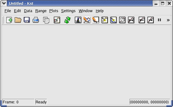
You can now start using KST! See Chapter 2 to start importing and working with data.
Currently, Kst supports ASCII text files, BOOMERANG frame files, and BLAST dirfile files as data sources. Additional file formats may be supported in the future.
The simplest input file format is the ASCII text file. These files are usually human-readable and can be created by hand if desired. The following is an example of an ASCII input file.
112.5 3776 428
187.5 5380 429
262.5 5245 345
337.5 2942 184
412.5 1861 119
487.5 2424 138
567.5 2520 162
637.5 1868 144
712.5 1736 211
787.5 1736 211
862.5 2172 292
937.5 1174 377
1000.5 499 623
Each column of this file represents a vector in KST. Columns are simply separated by spaces, and rows are separated by carriage returns.
The Data Wizard provides a quick and easy way of creating vectors, curves, and plots in KST from data files. To launch the wizard, select Data Wizard... from the Data menu. You will be prompted to select a data source. Browse to a valid data file (or enter in the path to a data file) and click Next. The following window will be displayed.
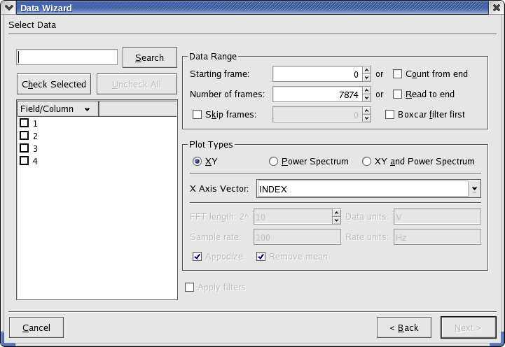
Select the fields you wish to import into KST. You may filter the list of fields by entering a string to match (wildcards are supported) into the text box above the list. The following list explains the selections and options available in the Data Range section.
- Starting frame
The first frame (row in the data file) to start reading data from.
- Count from end
Selecting this option reads the number of frames specified in Number of frames starting from the end of the data file.
- Number of frames
The total number of frames to read.
- Read to end
Selecting this option reads from the frame specified in Starting frame to the end of the file. Selecting both Count from end and Read to end has the effect of reading from the beginning to the end of the data file.
- Skip frames
The number of frames to skip when reading. For example, entering 1 for this field will cause every other frame to be skipped when reading from the data file.
- Boxcar filter first
Performs a boxcar filter first.
Power Spectrum and X axis settings can be specified within the Plot Types section. These settings are described below.
- XY, Power Spectrum, and XY and Power Spectrum
Select whether to plot the power spectrum (PSD) only, data only, or both. If the power spectrum is selected to be plotted, additional settings in this section become available.
- X Axis Vector
The vector to be used as the independent vector for the plots. You may select a field from your data file, or the INDEX vector. The INDEX vector is simply a vector containing elements from 0 to N-1, where N is the number of rows in the data file.
The remaining settings in the Plot Types section are available only if a power spectrum is to be plotted.
- FFT Length
The fast fourier transform length. The length is specified using the exponent x in 2^x.
- Data units
The units used for the data in the vectors.
- Rate units
The units to be used for the rate.
- Sample rate
The sample rate, using the units specified in Rate units.
- Appodize
Select this option to appodize the ends of the power spectrum.
- Remove Mean
Select this option to remove the mean from the selected data (i.e. translate the data so that the mean is zero).
Once you are satisfied with all the settings, click Next to advance to the next window. Select any filters you wish to apply to the data, and click Next to advance to the final window.
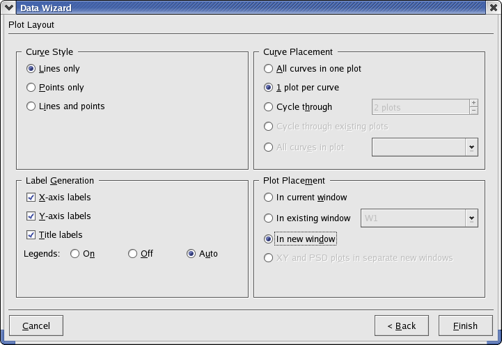
From here, you can change general plotting settings. Most of the settings are self-explanatory. A brief overview of each section is provided below.
- Curve Style
Select whether to plot data points only, lines connecting the data points only, or both.
- Curve Placement
Select the plots to place the new curves on. Cycle through creates the specified number of new plots and cycles through each plot, each time placing a new curve on the plot.
- Label Generation
Select the desired labels and legends to be placed on the plots.
- Plot Placement
Select the desired window(s) to place the new plots on. New windows can be created for the plots by selecting In new window.
Once you are satisfied with all the settings, click Finish and the plots will be generated.
The Data Manager provides a central location for adding, deleting, and modifying all the data objects used in KST. It can be accessed by selecting Data Manager from the Data menu.
To create a new data object from the Data Manager, click on one of the buttons listed under New:. A new window will be displayed, allowing options and settings for the data object to be set.
Tip
You can also create new curves by right-clicking on a vector and choosing Make Curve...
Since you are creating a new data object, you may enter a unique name to identify the object. The default name can be used as well (if it is unique).
The settings for all plottable data objects have two common sections—Curve Appearance and Curve Placement. These sections are described below. For data-specific settings, see Data Types.
Note
The “curves” referred to below are generally the visible lines and points on a plot when a data object is plotted—they do not in general refer to the “curve” data object.
The Curve Appearance section allows you to change the appearance of the data object when it is plotted.
-

Clicking this button displays a colour chooser dialog box, which can be used to change the colour of both the lines and points of the curve.
- Show points
Selecting this checkbox shows the data points used to plot the curve. The drop-down list to the right allows the shape of the points to be changed.
- Show lines
Selecting this checkbox shows the lines joining the data points for the curve. The thickness of the line as well as the line style can be changed.
The Curve Placement section specifies the location of new curves.
- Plot window
Specify the window to place the curve on. You may create a new window by clicking the New... button.
- Place in existing plot
Selecting this checkbox places a copy of the curve in an existing plot. Select the desired plot using the drop-down list to the right.
- Place in new plot
Selecting this checkbox places a copy of the curve in a new plot. Select the number of columns for the new plot. Note that you may place copies of the curve in both a new plot and an existing plot.
Once all the desired settings for the new data object have been set, click the Apply as New button to create the new data object.
To edit an existing data object, simply highlight it in the Data Manager window and click the Edit button. The settings window for the selected object will be displayed. This window is identical to the one displayed when creating new data objects, so refer to Creating New Data Objects for more information on the settings and options.
To delete a data object, highlight it in the Data Manager window and click the Delete button. Note that the entry in the # Used column for an object must be 0 before the object can be deleted. The # Used column indicates the number of times that a particular data object and its children (if any) are used by either other data object or by plots. Listed below are some consequences of this restriction to keep in mind when attempting to delete data objects.
All plottable objects (curves, equations, histograms, and power spectra) must be removed from plots before they can be deleted. An object can be removed from a plot by right-clicking on it in the Data Manager window and selecting the desired plot from the Remove From Plot submenu.
All curves that use a particular data vector must be deleted before the data vector can be deleted.
All children of a parent data object must be unused before the parent data object can be deleted.
After a sequence of deletions and removals of curves from plots, you may find that there are numerous unused data objects displayed in the Data Manager. To quickly remove these objects, you can click the Purge button.
There are seven main types of data objects in KST. Data objects can contain other data objects, as represented by the tree structure view in the Data Manager. The following diagram illustrates the relationships between the different data types.
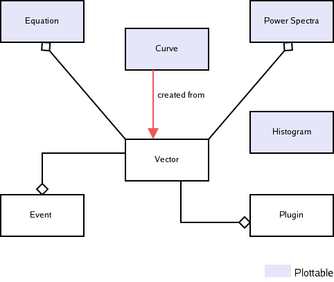
As can be seen from the above diagram, the curve, equation, histogram, and power spectra data objects are the only data objects that are plottable. Curves are created from vectors, while equations, power spectra, events, and plugins all contain slave vectors.
Descriptions of each data type are provided below, along with overviews of the settings and options available when creating or editing each type of data object. Settings common to almost all data types have been omitted—see Creating New Data Objects for more information.
Vectors are one of the most often-used data objects in KST. As their name implies, vectors are simply ordered lists of numbers. Most often they contain contain the x or y coordinates of a set of data points.
The following is a screenshot of the window displayed when creating or editing vectors. Explanations of the settings are listed below.
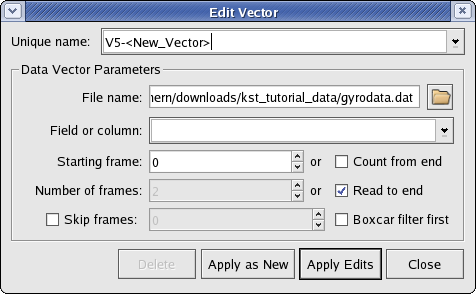
The source file and other parameters for the data vector can be set using the following options.
- Field or column
The field or column to create a vector from.
- Starting frame
The first frame (row in the data file) to start reading data from.
- Count from end
Selecting this option reads the number of frames specified in Number of frames starting from the end of the data file.
- Number of frames
The total number of frames to read.
- Read to end
Selecting this option reads from the frame specified in Starting frame to the end of the file. Selecting both Count from end and Read to end has the effect of reading from the beginning to the end of the data file.
- Skip frames
The number of frames to skip when reading. For example, entering 1 for this field will cause every other frame to be skipped when reading from the data file.
- Boxcar filter first
Performs a boxcar filter first.
Curves are primarily used to create plottable objects from vectors. Curves are created from two vectors - an “X axis vector” and a “Y axis vector”, that presumably provide a set of data points. Thus, a curve can be thought of as a set of data points and the lines that connect them.
The following is a screenshot of the window displayed when creating or editing curves. Explanations of the settings are listed below.
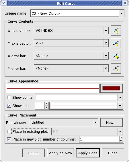
The contents of the curve can be set from this section.
- X axis vector
The vector to use for the independent (horizontal) axis.
- Y axis vector
The vector to use for the dependent (vertical) axis.
- X error bar
The vector containing error values corresponding to the X axis vector.
- Y error bar
The vector containing error values corresponding to the Y axis vector.
An equation data object consists of a mathematical expression and an independent variable. The expression is built using a combination of scalars, vectors, and operators, and usually represents the values of the dependent variable. The independent variable can be an existing vector or it can be generated when the equation object is created or edited. Since an equation ultimately consists of a set of data points, an equation object is plottable.
The following is a screenshot of the window displayed when creating or editing equations. Explanations of the settings are listed below.
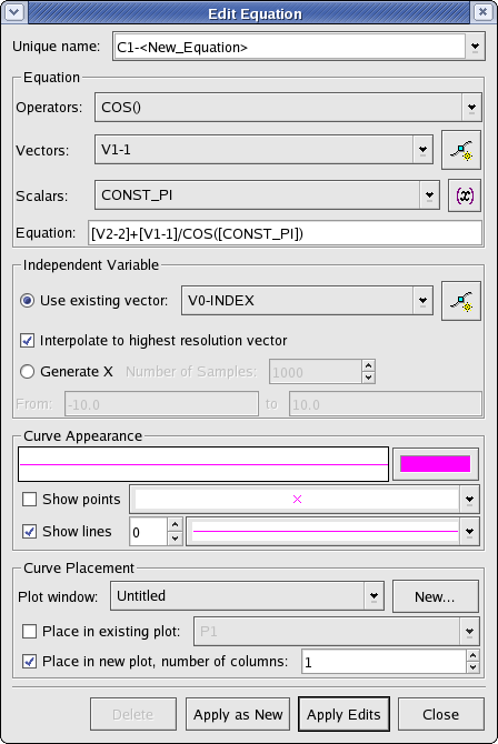
The mathematical expression representing the dependent variable can be modified from this section.
- Operators
A list of available operators. Choosing an operator from the list inserts the operator at the current insertion point in the Equation text box.
- Vectors
A list of the current vector objects in KST. Choosing a vector from the list inserts the vector at the current insertion point in the Equation text box.
- Scalars
A list of the available scalar values. This list is composed of both the scalar values in the current KST session as well as some built-in constants. Choosing a scalar from the list inserts the scalar at the current insertion point in the Equation text box.
- Equation
The mathematical expression representing the independent variable. You may manually type in this text box or you may select items to insert using the above drop-down lists.
This section is used to specify the source of the values for the independent variable.
- Use existing vector
A vector to use as the independent variable.
- Interpolate to highest resolution
Selecting this checkbox interpolates the existing vector the highest resolution possible.
- Generate X
Select this to generate a set of values to use as the independent variable. Specify the lowest value to generate in the From field, and the highest value to generate in the to field. Set the value for Number of samples to be the number of equally spaced values to generate between the lowest value and the highest value (inclusive).
A histogram data object simply represents a histogram of a particular vector. Histogram objects are plottable.
The following is a screenshot of the window displayed when creating or editing histograms. Explanations of the settings are listed below.
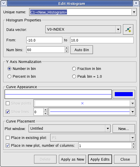
The source vector, as well as basic histogram properties, can be modified from this section.
- Data vector
The data vector to create the histogram from. Although a vector is needed to create a histogram, the vector is treated as an unordered set for the purposes of creating a histogram.
- From and to
The From field contains the left bound for the leftmost bin in the histogram. The to field contains the right bound for the rightmost bin in the histogram.
- Num bins
The number of bins for this histogram.
- Auto Bin
Clicking this button generates values for the From field and the to field based on the lowest and highest values found in the source vector, respectively.
This section is used to specify the type of normalization used for the y axis of the histogram.
- Number in bin
Selecting this option causes the y axis to represent the number of elements in each bin.
- Fraction in bin
Selecting this option causes the y axis to represent the fraction of elements (out of the total number of elements) in each bin.
- Percent in bin
Selecting this option causes the y axis to represent the percentage of elements (out of the total number of elements) in each bin.
- Peak bin = 1.0
Selecting this option causes the y axis to represent the number of elements in each bin divided by the number of elements in the largest bin (the bin with the greatest number of elements).
A power spectrum data object represents the power spectrum of a vector.
The following is a screenshot of the window displayed when creating or editing power spectra. Explanations of the settings are listed below.
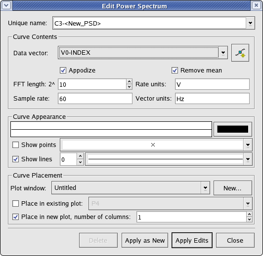
The source vector, as well as basic power spectrum properties, can be modified from this section.
- Data vector
The data vector create a power spectrum of.
- Appodize
Select this option to appodize the ends of the power spectrum.
- Remove Mean
Select this option to remove the mean from the selected data (i.e. translate the data so that the mean is zero).
- FFT Length
The fast fourier transform length. The length is specified using the exponent x in 2^x.
- Rate units
The units to be used for the rate.
- Sample rate
The sample rate.
A plugin data object represents a KST plugin. All plugins have a common format, and show up as type “Plugin” in the Data Manager. For more information about plugins, please see Plugins and Filters
An event data object represents an even monitor in KST. An event monitor essentially keeps track of one or more vectors or scalars, and performs a specified action when a specified condition involving the vectors or scalars is true. Event monitors are usually used in conjunction with “live”, or streaming data. For example, an event monitor could be created to monitor whether or not elements of a data vector representing temperature exceed a predefined value.
The following is a screenshot of the window displayed when creating or editing events. Explanations of the settings are listed below.
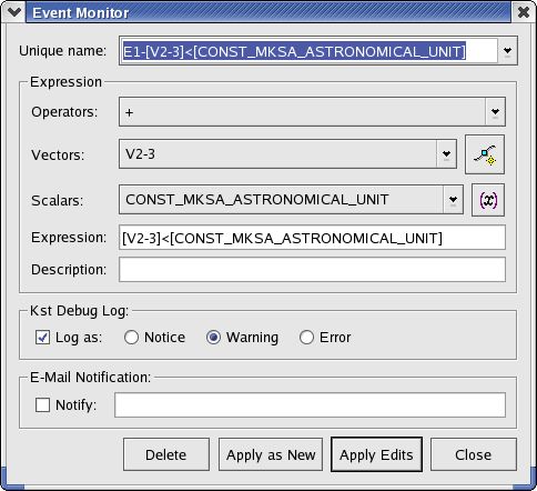
The condition to monitor for, along with other event properties, can be modified in this section.
- Operators
A list of available operators. Choosing an operator from the list inserts the operator at the current insertion point in the Expression text box.
- Vectors
A list of the current vector objects in KST. Choosing a vector from the list inserts the vector at the current insertion point in the Expression text box.
- Scalars
A list of the available scalar values. This list is composed of both the scalar values in the current KST session as well as some built-in constants. Choosing a scalar from the list inserts the scalar at the current insertion point in the Expression text box.
- Expression
The expression to monitor. You may type directly in this textbox, or select items to insert using the above drop-down lists. Ensure that the expression entered in this textbox is a boolean expression (i.e. it evaluates to either true or false). This usually entails using an equality or inequality in the expression. Note that vectors entered in the textbox will be monitored according to their individual elements.
Whenever this expression is true, the event will be triggered. The action taken upon an event trigger depends on the settings specified in the next two sections.
- Description
This textbox is used to store a short description of the event. The description is primarily available as a method for keeping track of multiple events. You can enter any text you wish in this textbox.
This section specifies settings for entries added to the KST debug log when events are triggered.
- Log as:
Enable this checkbox to have entries added to the KST debug log when this event is triggered.
- Notice
Log the entry as a notice.
- Warning
Log the entry as a warning.
- Error
Log the entry as an error.
The Data menu provides quick access to many features related to data objects in KST. Most of the menu functions duplicate functions found elsewhere, so only brief descriptions are provided below.
- Reload
Reloads all data vectors from their source files.
- Data Wizard...
Displays the Data Wizard.
- Data Manager
Displays the Data Manager.
- Edit [data object]
Displays the corresponding dialog for editing the data object. Refer to Data Types for descriptions of each dialog.
- View Scalars
Displays a dialog from which the values of all the scalars in the current KST session can be viewed. The dialog is updated dynamically if the values change.
- View Vectors
Displays a dialog from which the values in all the current vectors can be viewed. Select a vector to view using the drop-down list. The dialog is updated dynamically if the values change.
- Quickly Create New Curve
Displays a dialog for quickly creating new curve objects from data files. The dialog is a combination of the Edit Curve and Edit Vector dialogs.
- Quickly Create New PSD
Displays a dialog that allows quick creation of power spectrum objects from either data files or existing vectors. The dialog is a combination of the Edit Power Spectrum and Edit Vector dialogs.
- Change Data File
Displays a dialog for quickly changing data files that vectors are associated with. Select the vectors to change, and then browse to a different data file. Click Apply to save the changes.
This chapter details the concepts behind plots and windows, and provides information on viewing and manipulating the layout of plots and windows in KST. To clarify some terminology, the following diagram illustrates the relationships between windows, plots, and plottable data objects.
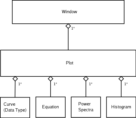
As can be seen from the above diagram, each window in KST can contain zero or more plots, and each plot can contain zero or more plottable data objects. One potentially confusing aspect of KST is that the terms “curve” and “plottable data object” are often used interchangeably. The easiest way to understand this is that “curve” and “plottable data object” are two different names for the same thing, and there also exists a data object that happens to be named “curve”. This data object also happens to be plottable, and thus it is a “curve” (in the first sense) as well. This anomoly in terminology should be kept in mind while reading the remaining sections in this chapter.
The plot dialog provides a central location for managing plots. To access it, select Edit Plots from the Plots menu. At the top of the dialog box you should see two drop-down lists:
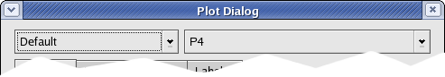
To modify a plot, select the window that contains from the plot from the left drop-down list, and select the plot itself from the right drop-down list.
At the bottom of the plot dialog are four buttons. The function of each button is listed below.
- Delete
Delete the currently selected plot. The plot will be removed from the window it previously resided in.
- Apply as New
Create a new plot using the current specified plot settings. Note that the plot must have a unique name (one which does not already exist).
- Apply Edits
Apply the specified plot settings to the currently selected plot.
- Close
Close the plot dialog.
The plot settings available on each tab of the plot dialog are described below.
Below is a screenshot of the Content tab.
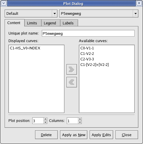
As the name implies, the settings on this tab specify the content of the plot. The following are brief explanations of the settings.
- Unique plot name
The unique plot name is the identifier for the plot. There cannot be duplicate plot names.
- Displayed curves and Available curves
Displayed curves lists the curves, or plottable data objects, that should be plotted in the plot. Available curves lists all the current plottable data objects in KST that are not in the Displayed curves list. To move a curve from one list to the other, first highlight the desired curve, and click the appropriate arrow button in between the two lists (the left arrow to move a curve from Available curves to Displayed curves, and the right arrow to move a curve from Displayed curves to Available curves).
- Plot position
The position of the plot in the window.
- Columns
The number of columns for the plot.
Below is a screenshot of the Limits tab.
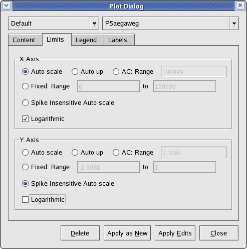
The settings for the plot axes are specified on this tab. The settings are split into two sections—an x axis section and a y axis section. The settings are identical between the two sections.
- Auto scale
Select this option to let KST automatically choose a scale for this axis based on the highest and lowest values for this axis found in the plotted curves.
- Auto up
I don't know what this does.
- AC
Select this option to have KST automatically choose a scale for the axis, based on the range limitation specified in Range.
- Fixed
Manually specify lower and upper limits for the axis. Enter the limits in the textboxes to the right of Range.
- Spike Insensitive Auto scale
Select this option to let KST automatically choose a scale for the axis that is not necessarily based on the highest and lowest values found in the plotted curves. In general, “spikes”, or sudden short increases or decreases in the value, will be ignored when determining the scale.
- Logarithmic
Enable this checkbox if you wish to use a logarithmic scale for the axis.
Below is a screenshot of the Legend tab.
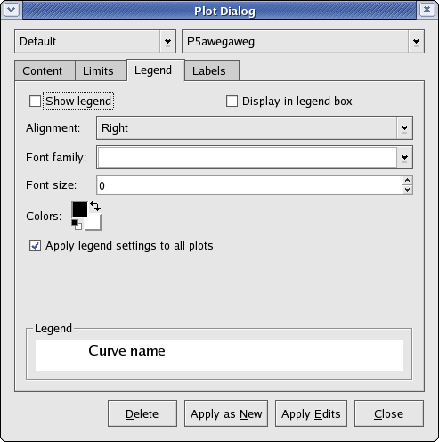
Legend settings for the plot can be specified on this tab; most of these settings concern the appearance of the legend. The legend itself is optional.
- Show legend
This option enables or disables the legend for the plot. If you wish to use a legend, you must select this checkbox.
- Display in legend box
Select this option to display a border around the legend.
- Alignment
The horizontal alignment of the items in the legend. The available settings in the drop-down list are Right, Center, and Left.
- Font family
The font to use for the legend text. Select a font from the drop-down list.
- Font size
The size of the legend text. Note that the size is not specified in points.
- Colors
This widget can be used to specify the colour of the legend text. The upper left box indicates the foreground colour, while the lower right box indicates the background colour (not currently used). To edit a colour, double-click on the desired box, and a standard colour chooser dialog will appear. Click
 to swap the foreground and background colours. If you wish to quickly return to the default colours, click

- Apply legend settings to all plots
If this checkbox is enabled, all the specified settings on this tab will be applied to every plot in KST when Apply as New or Apply Edits is clicked.
Note
Using this setting removes all previously specified legend settings for all plots.
- Legend (preview)
The preview image at the bottom of this tab provides a preview of what the legend text will look like at 100% zoom. Among other things, the preview can be useful in determining appropriate font sizes.
Below is a screenshot of the Labels tab.
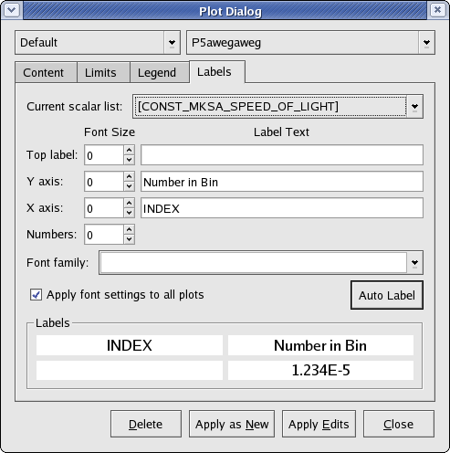
Settings for the plot labels can be specified on this tab. Brief descriptions of the settings are provided below.
- Current scalar list
A list of the current scalars defined in KST. This list is primarily used to quickly insert values in the label texts. Choosing an item from this list will insert the item at the current text cursor position.
- Top label
The label located at the top of the plot. Select a font size and enter the text for the label using the controls in this row.
- Y axis
The label located vertically next to the y axis of the plot. Select a font size and enter the text for the label using the controls in this row.
- X axis
The label located vertically next to the x axis of the plot. Select a font size and enter the text for the label using the controls in this row.
- Numbers
The numbers used to label both the x axis and the y axis of the plot. Only the size of the font can be specified.
- Font family
The font used for all labels of the plot. Select an available font using the drop-down list.
- Apply font settings to all plots
If this checkbox is enabled, the specified font family and font size settings will be applied to every plot in KST when Apply as New or Apply Edits is clicked.
Note
Using this setting removes all previously specified font family and font size settings on all plots. However, the actual label texts are not affected.
- Auto Label
Click this button to automatically generate label texts for all labels on the plot. The text for Top label will be a list of paths to the data files used in the plot. The text for Y axis will be a list of the dependent variable descriptions (e.g. “Number in Bin” for a histogram). The text for X axis will be the name of the vector used as the independent variable.
- Labels (preview)
The preview image at the bottom of the Labels tab provides previews of what all four labels will look like at 100% zoom.
When working with plots, right-clicking on any plot will bring up a context menu that provides commonly used functions. The following list provides a brief overview of the menu items, often referring to other sections of this document that describe the functions in more detail.
- Delete
Deletes the plot.
- Edit...
Brings up the Plot Dialog, with this plot selected. See the Plot Dialog section for information on the settings.
- Zoom
Expands the plot so that it takes up the entire area of the window. Uncheck this option to return the plot to its previous size.
- Pause
Pauses automatic update of live data. This menu item duplicates the functionality of Pause from the Range menu. See Working with Live Data for more information.
- Zoom (submenu)
The Zoom submenu is described in the section entitled The Zoom Menu.
- Scroll (submenu)
This menu is described in the section entitled The Scroll Menu.
- Edit (submenu)
This submenu displays a list of curves available for editing. Clicking on a curve name from the submenu displays the Edit Curve dialog for the curve. Details on this dialog are available in the Curves section.
- Fit (submenu)
This submenu displays a list of curves that can be fit. Selecting a curve name from the submenu displays the Fit Function dialog. This dialog is similar to the plugins dialog, but displays only those plugins that perform fits. The input vectors are selected based on the curve. In addition, visual curve properties can be selected, as the Fit function creates vectors, and curves based on the vectors.
- Remove (submenu)
This submenu displays a list of curves currently on the plot. Clicking on a curve name from the submenu removes the curve from the plot (the curve itself, however, is not removed as a data object).
The label editor allows custom labels to be placed in arbitrary locations in KST plot windows, in addition to the fixed labels created as part of plots. To use the label editor, select Label Editor from the Plots menu. The mouse mode will change to label editor mode. To exit label editor mode, select another mouse mode (such as XY Mouse Zoom). The following sections describe the functions available when in label editor mode.
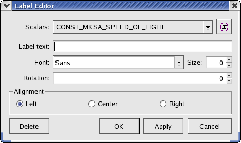
To create a new label using the label editor, click anywhere within the x and y axes of a plot where there is not already an existing label. The label editor dialog should appear:
The following are explanations of the dialog box elements.
- Scalars
A list of scalars currently defined in KST. Selecting an item from the dropdown list inserts the value of the item at the current cursor position in Label text.
- Label text
The text displayed by the label. You may enter text manually in this dialog and in combination with scalars selected from the Scalars dropdown list if you wish.
- Font
The font to use for the label text. Select a font from the dropdown list.
- Size
The size of the label text. 0 is the default value.
- Rotation
The number of degrees to rotate the label. Positive values rotate the label clockwise, while negative values rotate the label counter-clockwise.
- Alignment
The horizontal alignment of the label. Select one of Left, Center, or Right.
Once you are satisfied with the label settings, click Apply to apply the label settings without closing the label editor dialog. Click OK to apply the label settings and close the dialog. Alternatively, you can click Close to close the label editor dialog without applying any label settings.
To edit an existing label, click on the label in the plot. The label editor dialog should be displayed. You can delete the label from the label editor dialog by clicking the Delete button.
Data mode allows precise viewing of the data points use in a plotted curve. To toggle data mode, select Data Mode from the Plots menu. Now, when the cursor is moved over a plot, a red dot will indicate the closest data point to the cursor, as shown in the screenshot below. The status bar will display the coordinates of the data point (in terms of the x and y vectors used to plot the curve) in status bar at the lower right corner of the KST window. Note that all zooming functions are still available while in data mode.
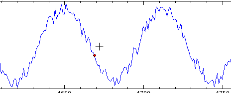
Tip
If the status bar is not visible, make sure Show Statusbar is checked in the Status menu.
Zooming and scrolling in plots is easy and intuitive with KST. The following sections explain the different zooming and scrolling modes.
To access the different zoom modes, choose one of XY Mouse Zoom, X Mouse Zoom, or Y Mouse Zoom from the Plots menu. The different modes are described below.
In XY Mouse Zoom mode, you can zoom into a specific rectangular area of the plot by simply clicking and dragging to draw a rectangle where desired. The x and y axes of the plot will change to reflect the new scale. This mode is often useful for quickly looking at an interesting area of the plot without having to specify exact axis scales.
In X Mouse Zoom mode, the y axis is fixed. Zooming in is performed by clicking and dragging a rectangular area; however, the upper and lower limits of the rectangle will always be equal to the current upper and lower limits of the y axis. This mode is often useful for looking at a certain time range, if the x axis happens to represent a time vector.
Tip
You can quickly switch to X Mouse Zoom mode by holding down Ctrl. The mouse cursor will change to indicate the new mode. Releasing Ctrl will return you to the previous mouse zoom mode.
In Y Mouse Zoom mode, the x axis is fixed. Zooming in is performed by clicking and dragging a rectangular area; however, the left and right limits of the rectangle will always be equal to the current left and right limits of the x axis. This mode is often useful for zooming in on data that is concentrated around a horizontal line.
Tip
You can quickly switch to Y Mouse Zoom mode by holding down Shift. The mouse cursor will change to indicate the new mode. Releasing Shift will return you to the previous mouse zoom mode.
The Zoom menu can be accessed by right-clicking on a plot and selecting the Zoom submenu from the context menu. A list of zoom actions and their corresponding keyboard shortcuts will be displayed. These actions are described below.
| Zoom Action | Keyboard Shortcut | Description |
|---|---|---|
| Zoom Maximum | M | Sets both the x axis and the y axis scales so that all data points are displayed. This is equivalent to the AutoScale setting of the Plot Dialog. |
| Zoom Max Spike Insensitive | S | Sets both the x axis and the y axis scales so that most data points are displayed. Spikes, or sudden increases or decreases in x or y values, are excluded from the plot display. |
| Zoom Previous | R | Returns to the most recent zoom setting used. |
| Y-Zoom AC Coupled | A | What is AC Coupled? |
| X-Zoom Maximum | Ctrl+M | Sets the x axis scale such that the x values for all data points are between the minimum and maximum of the x axis. The y axis scale is unaltered. |
| X-Zoom Out | Shift+Right | For a non-logarithmic x axis, increases the length of the x axis by a factor of approximately 0.5, without changing the midpoint of the x axis. The y axis scale is unaltered. |
| X-Zoom In | Shift+Left | For a non-logarithmic x axis, decreases the length of the x axis by a factor of approximately 0.5, without changing the midpoint of the x axis. The y axis scale is unaltered. |
| Toggle Log X Axis | G | Enables or disables using a logarithmic scale for the x axis. |
| Y-Zoom Maximum | Shift+M | Sets the y axis scale such that the y values for all data points are between the minimum and maximum of the y axis. The x axis scale is unaltered. |
| Y-Zoom Out | Shift+Up | For a non-logarithmic y axis, increases the length of the y axis by a factor of approximately 0.5, without changing the midpoint of the y axis. The x axis scale is unaltered. |
| Y-Zoom In | Shift+Down | For a non-logarithmic y axis, decreases the length of the y axis by a factor of approximately 0.5, without changing the midpoint of the y axis. The x axis scale is unaltered. |
| Toggle Log Y Axis | L | Enables or disables using a logarithmic scale for the y axis. |
Many of the zoom actions are best used in conjunction with the various mouse zoom modes.
To quickly change the axes of a plot to match those of another plot, right-click on the plot and select a different plot name from the Match Axis... menu. Both the x and y axes scales of the current plot will change to match those of the selected plot. Note that this does not permanently tie the axes scales together; changing the zoom on either plot will unmatch the axes scales again. To tie the axes scales of two or more plots together, use the Tied Zoom feature.
Functions for scrolling a plot are available by right-clicking a plot and selecting the Scroll submenu from the context menu. The scrolling functions and their keyboard shortcuts should be self-explanatory. Assuming non-logarithmic axis scales are used, each function scrolls the plot in the indicated direction by 0.1 of the current length of the x axis (when scrolling left or right), or 0.25 of the current length of the y axis (when scrolling up or down).
Tip
To quickly go forwards or backwards along the x axis, select Back 1 Screen or Advance 1 Screen from the Range menu. The keyboard shortcuts, Ctrl+Left and Ctrl+Right respectively, can be used as well.
When looking at two or more related plots (for example, two curves on separate plots both dependent on the same time vector), it can sometimes be useful to zoom or scroll the plots simultaneously. This is possible using KST's tied zoom feature. To activate tied zoom, click the small square at the top-right corner of the plots you wish to tie together. The squares will turn black in colour to indicate the plots are tied, as shown below.
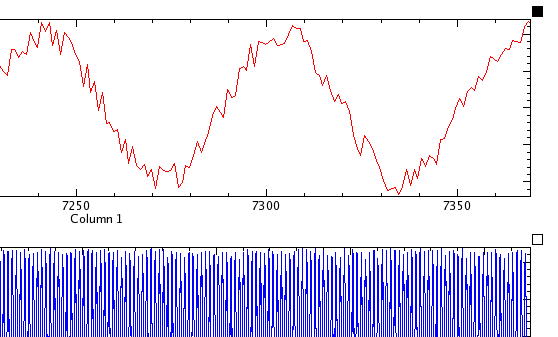
Zooming and scrolling actions performed on one plot in a group of tied plots will be performed on on all the plots in the group. To remove a plot from the tied group, simply click on the small square at the top-right corner of the plot again. The square will turn white in colour to indicate the plot is not tied.
KST features special zooming and scrolling functions designed to make it easy to work with “live” data, or data that is being updated while KST is running. These features are designed to be used in conjunction with the regular zooming and scrolling functions.
To have a plot automatically update as data is being added to a data file, choose Read From End from the Range menu. The plot will automatically scroll to the right periodically, to display new data points. The update interval can be changed by selecting Configure Kst... from the Settings menu. Specify the update interval in the Plot Update Timer field.
To pause automatic updating of plots, select Pause from the Range menu. You can still perform zooming and scrolling functions while the updating is paused. Selecting Read From End from the Range menu will resume automatic updating.
To quickly change sample range settings associated with vectors, select Change Data Sample Ranges from the Range menu. Select one or more vectors, change the desired settings for the vectors, and click Apply to save the settings. These settings are a subset of those found in the Edit Vectors dialog.
Plots in a KST window are arranged in layers. Each plot is positioned on one layer, and each layer contains one plot. Thus, plots can overlap, with plots in higher layers taking precedence in visibility over those in lower ones. To change the layout of plots in KST, layout mode must be activated. Layout mode can be toggled by selecting Layout Mode from the Plots menu.
While layout mode is activated, right-clicking on any plot displays a modified context menu. The selections available in this menu are listed below.
- Delete
Deletes the plot.
- Raise
Raises the plot one layer up.
- Lower
Lowers the plot one layer down.
- Raise to Top
Raises the plot to the top-most layer, guaranteeing it will be visible.
- Lower to Bottom
Lowers the plot to the bottom-most layer.
- Rename...
Selecting this item displays a dialog box that allows the unique name of the plot to be changed.
- Cleanup Layout
Arranges the plots in the current window in a tile type pattern, with no overlap between plots. This action applies to all plots in the current window.
Moving and resizing plots in layout mode is analogous to moving and resizing regular windows. To move a plot, simply click anywhere on the desired plot and drag the plot. An outline of the plot will appear, indicating where the plot will be placed. You can drag plots anywhere within the current window. To resize a plot, move the mouse cursor to the any edge or corner of the plot. The cursor will change to indicate that the plot can be resized. Click and drag the outline of the plot until the plot is the desired shape and size.
KST has a flexible window layout that makes use of Kmdi. Organizing plots on different windows allows for efficient viewing and manipulating of plots.
There is a choice of four different MDI (Multi-Document Interface) modes available. To select a mode, choose one of the menu items from the MDI Mode... submenu of the Window menu. The selected MDI mode will take effect immediately. The sections below provide more information on each mode.
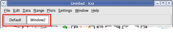
Top level mode is the mode traditionally used by other KDE applications. In this mode, the parent window (the window containing all the main menus, toolbars, and status bars) is a separate window from the plot windows. The plot windows, while still functionally tied to the main window, appear as separate windows on the desktop.
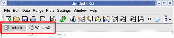
To quickly switch between plot windows in top level mode, you can click the buttons on the parent window, as shown below.
In childframe mode, all the plot windows appear inside the main KST window and can be individually resized. Each plot window contains buttons for minimizing, maximizing, closing, and docking themselves. The main KST window also contains functions for arranging the plot windows. The following lists the functionality of the buttons located in the top right corner of each plot window:

Undocks the plot window. An undocked window is not contained within the main KST window, but is located directly on the desktop.
Tip
You can also undock or dock a window by selecting its name from the Dock/Undock submenu of the Window menu. This is also the only way to dock an undocked window.

Minimizes the plot window. Since the plot window is contained within the main KST window, clicking this button will minimize the window to a titlebar within the KST window.

Maximizes the plot window. The plot window will take up the entirety of the main KST window.

Closes the plot window.
To quickly switch between plot windows in childframe mode, you can click the buttons on the parent window, as shown below.
To easily organize the plot windows within the main KST window, you can choose one of the tiling functions from the Tile... submenu of the Window menu. These functions are described below.
- Cascade Windows
Cascades the windows starting from the top left corner, maintaining the original window sizes.
- Cascade Windows
Cascades the windows starting from the top left corner, but resizes each window so that the bottom right corner of each window reaches the bottom right of the main KST window.
- Expand Vertically
Resizes each window to its maximum height. The widths of the windows are not changed.
- Expand Horizontally
Resizes each window to its maximum width. The heights of the windows are not changed.
- Tile Non-overlapped
Arranges the windows in a tile pattern, with no windows overlapping and each window being as close to a square as possible.
- Tile Overlapped
Arranges the windows in three or four stacks, depending on the number of windows and the main KST window size.
- Tile Vertically
Arranges the windows in a tile pattern, with each window having maximum height and no windows overlapping.
Tab page mode arranges each plot window on a separate tab within the main KST window. In this mode, the plot windows are not independently resizeable or moveable—they conform to the size and shape of the main KST window.
To switch between plot windows in tab page mode, you can click on the tabs corresponding to each window, as shown below.
New windows in KST can be created in a number of ways. To create a new, empty, window, select New Window from the File menu. You will be prompted for a unique name for the new window. You can also create a new window while creating a new plottable data object. See Curve Placement for the specific details.
To delete an existing window, simply select Close from the Window menu. To delete all current windows in KST, select Close All from the Window menu.
Important
When a window is deleted, all plots within that window are deleted as well. However, data objects, such as curves, are not deleted.
KST provides various methods of saving and exporting data and plots. These methods are described below.
A plot definition is essentially a capture of a KST session. It contains all the plots, data objects, and plot layouts that are present at the time of saving.
To save a plot definition, simply select Save or Save As... (depending on whether or not you wish to save to a new file) from the File menu. Browse to the location you wish to save the plot definition, enter a filename, and click Save. The plot definition will be saved as a *.kst file.
Vectors and plots in KST can be exported to files. This can be useful, for example, in capturing plots of live data or using generated vectors in a different application.
To export or save a vector to a file, select Save Vectors to Disk... from the File menu. The vector will be saved as an ASCII data file. The first column of the file will contain an automatically generated index vector, starting a 0, while the second column of the file will contain the elements of the selected vector. See below for an example of an exported vector.
0 3776
1 5380
2 5245
3 2942
4 1861
5 2424
6 2520
7 1868
8 1736
9 1736
10 2172
11 1174
12 499
To export a KST plot to a graphics file, select Export to Graphics File... from the File menu. The following dialog box will appear.
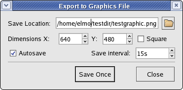
The following settings and options are available when saving:
- Save location
The location to save the graphics file. Enter a location manually, or click the button to right of the text box to browse to a location.
- Dimensions
Select the dimensions, in pixels, of the graphic. Check the Square option if you wish for the length and width of the graphic to be equal.
- Autosave
Check this option if you want KST to automatically save the plot to the specified file on a specified time interval.
- Save interval
The time interval used to perform autosave, in seconds.
Click Save Once to immediately perform a save with the specified options and settings. Click Close to close the dialog box (autosave will still be performed, if specified).
To print all the plots in the current window, select Print... from the File menu. A standard KDE print dialog will be displayed. There are currently no options to select for printing. The printed page will be in landscape orientation and contain the arrangement of plots in the current window. A footer containing the page number, window name, and current date is included as well.
Plugins and filters provide added functionality to KST. By default, KST comes packaged with an extensive selection of built-in plugins. In addition, a simple and consistent interface allows for easy creation of 3rd-party plugins.
By default, the built-in plugins are stored in /usr/lib/kde3/kstplugins/ (this directory may vary, depending on where you installed KST). The Plugin Manager can be used to add and remove plugins. It can be acccessed by selecting Plugins... from the Settings menu. A list of the currently installed plugins is displayed in the Plugin Manager.
To add a plugin, click the Install... button. Browse to the directory containing both the plugin specification file (*.xml) and the object file (*.o). Click OK, and the plugin should be installed.
To remove a plugin, simply highlight the plugin in the Plugin Manager and click Remove. You will be prompted for confirmation.
To quickly refresh the list of plugins displayed in the Plugin Manager, click Rescan. Doing so will remove any plugins no longer present in their specified paths, and add any new plugins in the default plugins directory.
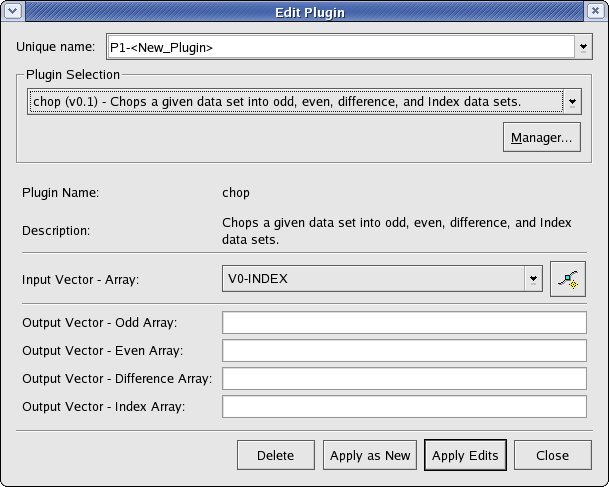
To date, there are more than 25 built-in plugins available in KST that perform functions from taking cross correlations of two vectors to producing periodograms of a data set. The settings window for every plugin consists of two main sections—an input section and an output section. Each section is composed of a set of scalars and/or vectors. The following screenshot shows the settings window for a typical plugin. The only difference between the different plugins is the set of inputs and outputs, and the mechanism for deriving the outputs from the inputs.
The following sections describe the purpose, key algorithms or formulas used to perform calculations, and inputs and outputs for each plugin.
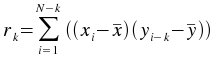
The autocorrelation plugin calculates correlation values between a series (vector) and a lagged version of itself, using lag values from floor(-(N-1)/2) to floor((N-1)/2), where N is the number of points in the data set. The time vector is not an input as it is assumed that the data is sampled at equal time intervals. The correlation value r at lag k is:
The bin plugin bins elements of a single data vector into bins of a specified size. The value of each bin is the mean of the elements belonging to the bin. For example, if the bin size is 3, and the input vector is [9,2,7,3,4,74,5,322,444,2,1], then the outputted bins would be [6,27,257]. Note that any elements remaining at the end of the input vector that do not form a complete bin (in this case, elements 2 and 1), are simply discarded.
The convolution plugin generates the convolution of one vector with another. The convolution of two functions f and g is given by:
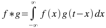
The order of the vectors does not matter, since f*g=g*f. In addition, the vectors do not need to be of the same size, as the plugin will automatically extrapolate the smaller vector.
- Array One (vector)
One of the pair of arrays to take the convolution of.
- Array Two (vector)
One of the pair of arrays to take the convolution of.
The deconvolution plugin generates the deconvolution of one vector with another. Deconvolution is the inverse of convolution. Given the convolved vector h and another vector g, the deconvolution f is given by:

The vectors do not need to be of the same size, as the plugin will automatically extrapolate the shorter vector. The shorter vector is assumed to be the response function g.
- Array One (vector)
One of the pair of arrays to take the deconvolution of.
- Array Two (vector)
One of the pair of arrays to take the deconvolution of.
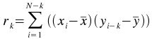
The crosscorrelation plugin calculates correlation values between two series (vectors) x and y, using lag values from floor(-(N-1)/2) to floor((N-1)/2), where N is the number of elements in the longer vector. The shorter vector is padded to the length of the longer vector using 0s. The time vector is not an input as it is assumed that the data is sampled at equal time intervals. The correlation value r at lag k is:
- X Array (vector)
The array x used in the cross-correlation formula.
- Y Array (vector)
The array y used in the cross-correlation formula.
The chop plugin takes an input vector and divides it into two vectors. Every second element in the input vector is placed in one output vector, while all other elements from the input vector are placed in another output vector.
- Odd Array (vector)
The array containing the odd part of the input array (i.e. it contains the first element of the input array).
- Even Array (vector)
The array containing the even part of the input array (i.e. it does not contain the first element of the input array).
- Difference Array (vector)
The array containing the elements of the odd array minus the respective elements of the even array.
- Index Array (vector)
An index array the same length as the other three output arrays.
The kstfit_linear_weighted plugin performs a weighted least-squares fit to a straight line model:

The best-fit is found by minimizing the weighted sum of squared residuals:
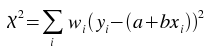
for a and b, where wi is the weight at index i.
- X Array (vector)
The array of x values for the data points to be fitted.
- Y Array (vector)
The array of y values for the data points to be fitted.
- Weights (vector)
The array containing weights to be used for the fit.
- Y Fitted (vector)
The array of y values for the points representing the best-fit line.
- Residuals (vector)
The array of residuals, or differences between the y values of the best-fit line and the y values of the data points.
- Parameters (vector)
The parameters a and b of the best-fit.
- Covariance (vector)
The estimated covariance matrix, returned row after row, starting with row 0.
- Y Lo (vector)
The corresponding value in Y Fitted minus the standard deviation of the best-fit function at the corresponding x value.
- Y Hi (vector)
The corresponding value in Y Fitted plus the standard deviation of the best-fit function at the corresponding x value.
- chi^2/nu (scalar)
The value of the sum of squares of the residuals, divided by the degrees of freedom.
The kstfit_linear_unweighted plugin is identical in function to the kstfit_linear_weighted plugin with the exception that the weight value wi is equal to 1 for all index values i. As a result, the Weights (vector) input does not exist.
The kstfit_gradient_weighted plugin performs a weighted least-squares fit to a straight line model without a constant term:

The best-fit is found by minimizing the weighted sum of squared residuals:
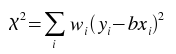
for b, where wi is the weight at index i.
- X Array (vector)
The array of x values for the data points to be fitted.
- Y Array (vector)
The array of y values for the data points to be fitted.
- Weights (vector)
The array containing weights to be used for the fit.
- Y Fitted (vector)
The array of y values for the points representing the best-fit line.
- Residuals (vector)
The array of residuals, or differences between the y values of the best-fit line and the y values of the data points.
- Parameters (vector)
The parameter b of the best-fit.
- Covariance (vector)
The estimated covariance matrix, returned row after row, starting with row 0.
- Y Lo (vector)
The corresponding value in Y Fitted minus the standard deviation of the best-fit function at the corresponding x value.
- Y Hi (vector)
The corresponding value in Y Fitted plus the standard deviation of the best-fit function at the corresponding x value.
- chi^2/nu (scalar)
The value of the sum of squares of the residuals, divided by the degrees of freedom.
The kstfit_linear_unweighted plugin is identical in function to the kstfit_gradient_weighted plugin with the exception that the weight value wi is equal to 1 for all index values i. As a result, the Weights (vector) input does not exist.
The statistics plugin calculates statistics for a given data set. Most of the output scalars are named such that the values they represent should be apparent. Standard formulas are used to calculate the statistical values.
- Mean (scalar)
The mean of the data values.
- Minimum (scalar)
The minimum value found in the data array.
- Maximum (scalar)
The maximum value found in the data array.
- Variance (scalar)
The variance of the data set.
- Standard deviation (scalar)
The standard deviation of the data set.
- Median (scalar)
The median of the data set.
- Absolute deviation (scalar)
The absolute deviation of the data set.
- Skewness (scalar)
The skewness of the data set. (what kind? formula?)
- Kurtosis (scalar)
The kurtosis of the data set. (what kind? formula?)
The kstfit_polynomial_weighted plugin performs a weighted least-squares fit to a polynomial model:
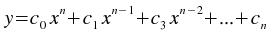
where n is the degree of the polynomial model.
- X Array (vector)
The array of x values for the data points to be fitted.
- Y Array (vector)
The array of y values for the data points to be fitted.
- Weights (vector)
The array of weights to use for the fit.
- Order (scalar)
The order, or degree, of the polynomial model to use.
- Y Fitted (vector)
The array of fitted y values.
- Residuals (vector)
The array of residuals.
- Parameters (vector)
The best fit parameters c0, c1,..., cn.
- Covariance (vector)
The covariance matrix of the model parameters, returned row after row in the vector.
- chi^2/nu (scalar)
The weighted sum of squares of the residuals, divided by the degrees of freedom.
The kstfit_polynomial_unweighted plugin is identical in function to the kstfit_polynomial_weighted plugin with the exception that the weight value wi is equal to 1 for all index values i. As a result, the Weights (vector) input does not exist.
The kstfit_sinusoid_weighted plugin performs a least-squares fit to a sinusoid model:

where T is the specified period, and n=2+2H, where H is the specified number of harmonics.
- X Array (vector)
The array of x values for the data points to be fitted.
- Y Array (vector)
The array of y values for the data points to be fitted.
- Weights (vector)
The array of weights to use for the fit.
- Harmonics (scalar)
The number of harmonics of the sinusoid to fit.
- Period (scalar)
The period of the sinusoid to fit.
- Y Fitted (vector)
The array of fitted y values.
- Residuals (vector)
The array of residuals.
- Parameters (vector)
The best fit parameters c0, c1,..., cn.
- Covariance (vector)
The covariance matrix of the model parameters, returned row after row in the vector.
- chi^2/nu (scalar)
The weighted sum of squares of the residuals, divided by the degrees of freedom.
The kstfit_sinusoid_unweighted plugin is identical in function to the kstfit_sinusoid_weighted plugin with the exception that the weight value wi is equal to 1 for all index values i. As a result, the Weights (vector) input does not exist.
The kstfit_exponential_weighted plugin performs a weighted non-linear least-squares fit to an exponential model:
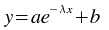
An initial estimate of
a=1.0,
 =0, and
b=0 is used. The plugin subsequently iterates to the solution
until a precision of 1.0e-4 is reached or 500 iterations have been performed.
=0, and
b=0 is used. The plugin subsequently iterates to the solution
until a precision of 1.0e-4 is reached or 500 iterations have been performed.
- X Array (vector)
The array of x values for the data points to be fitted.
- Y Array (vector)
The array of y values for the data points to be fitted.
- Weights (vector)
The array of weights to use for the fit.
- Y Fitted (vector)
The array of fitted y values.
- Residuals (vector)
The array of residuals.
- Parameters (vector)
The best fit parameters a,
, and
b.
- Covariance (vector)
The covariance matrix of the model parameters, returned row after row in the vector.
- chi^2/nu (scalar)
The weighted sum of squares of the residuals, divided by the degrees of freedom.
The kstfit_exponential_unweighted plugin is identical in function to the kstfit_exponential_weighted plugin with the exception that the weight value wi is equal to 1 for all index values i. As a result, the Weights (vector) input does not exist.
The kstfit_gaussian_weighted plugin performs a weighted non-linear least-squares fit to a Gaussian model:
An initial estimate of
a=(maximum of the y values),
 =(mean of the x values), and
 =(the midpoint of the x values)
is used. The plugin subsequently iterates to the solution
until a precision of 1.0e-4 is reached or 500 iterations have been performed.
=(the midpoint of the x values)
is used. The plugin subsequently iterates to the solution
until a precision of 1.0e-4 is reached or 500 iterations have been performed.
- X Array (vector)
The array of x values for the data points to be fitted.
- Y Array (vector)
The array of y values for the data points to be fitted.
- Weights (vector)
The array of weights to use for the fit.
- Y Fitted (vector)
The array of fitted y values.
- Residuals (vector)
The array of residuals.
- Parameters (vector)
The best fit parameters
,
, and
a.
- Covariance (vector)
The covariance matrix of the model parameters, returned row after row in the vector.
- chi^2/nu (scalar)
The weighted sum of squares of the residuals, divided by the degrees of freedom.
The kstfit_gaussian_unweighted plugin is identical in function to the kstfit_gaussian_weighted plugin with the exception that the weight value wi is equal to 1 for all index values i. As a result, the Weights (vector) input does not exist.
The kstfit_lorentzian_weighted plugin performs a weighted non-linear least-squares fit to a Lorentzian model:
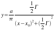
An initial estimate of
a=(maximum of the y values),
x0=(mean of the x values), and
 =(the midpoint of the x values)
is used. The plugin subsequently iterates to the solution
until a precision of 1.0e-4 is reached or 500 iterations have been performed.
=(the midpoint of the x values)
is used. The plugin subsequently iterates to the solution
until a precision of 1.0e-4 is reached or 500 iterations have been performed.
- X Array (vector)
The array of x values for the data points to be fitted.
- Y Array (vector)
The array of y values for the data points to be fitted.
- Weights (vector)
The array of weights to use for the fit.
- Y Fitted (vector)
The array of fitted y values.
- Residuals (vector)
The array of residuals.
- Parameters (vector)
The best fit parameters x0,
, and
a.
- Covariance (vector)
The covariance matrix of the model parameters, returned row after row in the vector.
- chi^2/nu (scalar)
The weighted sum of squares of the residuals, divided by the degrees of freedom.
The kstfit_lorentzian_unweighted plugin is identical in function to the kstfit_lorentzian_weighted plugin with the exception that the weight value wi is equal to 1 for all index values i. As a result, the Weights (vector) input does not exist.
The kstinterp_akima plugin generates a non-rounded Akima spline interpolation for the supplied data set, using natural boundary conditions.
- X Array (vector)
The array of x values of the data points to generate the interpolation for.
- Y Array (vector)
The array of y values of the data points to generate the interpolation for.
- X' Array (vector)
The array of x values for which interpolated y values are desired.
The kstinterp_akima_periodic plugin generates a non-rounded Akima spline interpolation for the supplied data set, using periodic boundary conditions.
- X Array (vector)
The array of x values of the data points to generate the interpolation for.
- Y Array (vector)
The array of y values of the data points to generate the interpolation for.
- X' Array (vector)
The array of x values for which interpolated y values are desired.
The kstinterp_cspline plugin generates a cubic spline interpolation for the supplied data set, using natural boundary conditions.
- X Array (vector)
The array of x values of the data points to generate the interpolation for.
- Y Array (vector)
The array of y values of the data points to generate the interpolation for.
- X' Array (vector)
The array of x values for which interpolated y values are desired.
The kstinterp_cspline_periodic plugin generates a cubic spline interpolation for the supplied data set, using periodic boundary conditions.
- X Array (vector)
The array of x values of the data points to generate the interpolation for.
- Y Array (vector)
The array of y values of the data points to generate the interpolation for.
- X' Array (vector)
The array of x values for which interpolated y values are desired.
The kstinterp_linear plugin generates a linear interpolation for the supplied data set.
- X Array (vector)
The array of x values of the data points to generate the interpolation for.
- Y Array (vector)
The array of y values of the data points to generate the interpolation for.
- X' Array (vector)
The array of x values for which interpolated y values are desired.
The kstinterp_polynomial plugin generates a polynomial interpolation for the supplied data set. The number of terms in the polynomial used is equal to the number of points in the supplied data set.
- X Array (vector)
The array of x values of the data points to generate the interpolation for.
- Y Array (vector)
The array of y values of the data points to generate the interpolation for.
- X' Array (vector)
The array of x values for which interpolated y values are desired.
The periodogram plugin produces the periodogram of a given data set. One of two algorithms is used depending on the size of the data set—a fast algorithm is used if there are greater than 100 data points, while a slower algorithm is used if there are less than or equal to 100 data points.
- Time Array (vector)
The array of time values of the data points to generate the interpolation for.
- Data Array (vector)
The array of data values, dependent on the time values, of the data points to generate the interpolation for.
- Oversampling factor (scalar)
The factor to oversample by.
- Average Nyquist frequency factor (scalar)
The average Nyquist frequency factor.
The following are descriptions of the filters built in to KST.
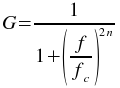
The butterworth_bandpass plugin filters a set of data with a Butterworth band pass filter. The filtering is performed by calculating the Fourier transform of the data and recalculating the the frequency responses using the following formula
where f is the frequency, fc is the low frequency cutoff, b is the bandwidth of the band to pass, and n is the order of the Butterworth filter. The inverse Fourier transform is then calculated using the new filtered frequency responses.
- X Array (vector)
The array of values to filter.
- Order (scalar)
The order of the Butterworth filter to use.
- Low cutoff frequency (scalar)
The low cutoff frequency of the Butterworth band pass filter.
- Band width (scalar)
The width of the band to pass. This should be the difference between the desired high cutoff frequency and the low cutoff frequency.
The butterworth_bandstop plugin filters a set of data with a Butterworth band stop filter. The filtering is performed by calculating the Fourier transform of the data and recalculating the the frequency responses using the following formula
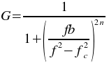
where f is the frequency, fc is the low frequency cutoff, b is the bandwidth of the band to stop, and n is the order of the Butterworth filter. The inverse Fourier transform is then calculated using the new filtered frequency responses.
- X Array (vector)
The array of values to filter.
- Order (scalar)
The order of the Butterworth filter to use.
- Low cutoff frequency (scalar)
The low cutoff frequency of the Butterworth band stop filter.
- Band width (scalar)
The width of the band to stop. This should be the difference between the desired high cutoff frequency and the low cutoff frequency.
The butterworth_highpass plugin filters a set of data with a Butterworth high pass filter. The filtering is performed by calculating the Fourier transform of the data and recalculating the the frequency responses using the following formula
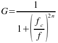
where f is the frequency, fc is the high frequency cutoff, and n is the order of the Butterworth filter. The inverse Fourier transform is then calculated using the new filtered frequency responses.
- X Array (vector)
The array of values to filter.
- Order (scalar)
The order of the Butterworth filter to use.
- Cutoff frequency (scalar)
The cutoff frequency of the Butterworth high pass filter.
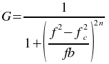
The butterworth_lowpass plugin filters a set of data with a Butterworth low pass filter. The filtering is performed by calculating the Fourier transform of the data and recalculating the the frequency responses using the following formula
where f is the frequency, fc is the low frequency cutoff, and n is the order of the Butterworth filter. The inverse Fourier transform is then calculated using the new filtered frequency responses.
- X Array (vector)
The array of values to filter.
- Order (scalar)
The order of the Butterworth filter to use.
- Cutoff frequency (scalar)
The cutoff frequency of the Butterworth low pass filter.
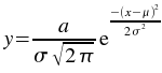
The noise addition plugin adds a Gaussian random variable to each element of the input vector. The Gaussian distribution used has a mean of 0 and the specified standard deviation. The probability density function of a Gaussian random variable is:
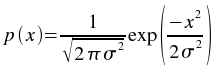
- Array (vector)
The array of elements to which random noise is to be added.
- Sigma (scalar)
The standard deviation to use for the Gaussian distribution.
This chapter describes miscellaneous time-saving and convenience features available in KST.
The toolbar provides one-click access to commonly used menu functions in KST. To toggle the toolbar, select Show Toolbar from the Settings menu.
The toolbar menu, accessible by right-clicking anywhere on the toolbar, contains functions for modifying the layout, appearance, and behaviour of the toolbar. The three submenus available are described below.
The Orientation submenu contains layout options for the toolbar.
- Top
Docks the toolbar at the top edge of the KST window.
- Left
Docks the toolbar at the left edge of the KST window.
- Right
Docks the toolbar at the right edge of the KST window.
- Bottom
Docks the toolbar at the bottom edge of the KST window.
- Flat
Hides the toolbar and turns it into a slim bar at the top of KST window. To unhide the toolbar, click on the “gripper” that is still visible.
You can also move the toolbar by dragging the gripper on the edge of the toolbar. Dragging the toolbar close to an edge of the KST window docks it. Dragging the toolbar anywhere else turns it into a floating toolbar.
The Text Position submenu specifies if and how text and icons should be displayed on the toolbar.
- Icons Only
Does not display any text labels and only displays icons. However, the text for each icon is still available as a tooltip associated with the icon (viewable by momentarily holding the cursor of the icon).
- Text Only
Does not display any icons on the toolbar, but displays all text labels.
- Text Alongside Icons
Displays all icons. Text labels are displayed to the right of the icons.
- Text Under Icons
Displays all icons. Text labels are displayed underneath the icons.
The Icon Size submenu specifies the size of the icons on the toolbar. The options in this menu do not have any effect if Text Only is selected for Text Position.
- Default
Uses the default size for each icon on the toolbar.
- Small (16x16)
Sizes each icon on the toolbar to a 16x16 pixel square.
- Medium (22x22)
Sizes each icon on the toolbar to a 22x22 pixel square.
- Large (32x32)
Sizes each icon on the toolbar to a 32x32 pixel square.
You can create custom shortcut keys to make working in KST more efficient. To modify the shortcut keys, select Configure Shortcuts... from the Settings menu. The following dialog will be displayed.
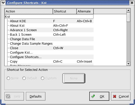
A list of available actions and their associated shortcuts are shown in the dialog. Each action is allowed two shortcuts—a primary shortcut and an alternate shortcut. Either shortcut can be used at any time. To define or change a shortcut for an action, simply highlight the appropriate row in the shortcut list. Under Shortcut for Selected Action, there are three choices:
- None
Select this option to disable any shortcut keys for the selected action.
- Default
Select this option to use the default shortcut key(s) for the selected action. Note that not all actions have default shortcuts defined.
- Custom
Select this option to define a custom shortcut for the selected action.
If you select the Custom option, the Define Shortcut dialog will appear (alternatively, you can also click on the key-shaped button next to the right to open the dialog).
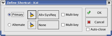
By default, the Auto-close option is checked, so once a key combination is entered, the key combination will be automatically saved and the dialog closed. You can uncheck this option if you wish to experiment with the dialog.
To define a key combination, select Primary or Alternate. If you wish to define a key sequence, check the Multi-key option. Now enter the key combination or sequence to be used for this action. Click OK when you are done.
Tip
When using shortcuts defined with the multi-key option, a small menu is displayed after the first key of the shortcut is pressed, showing the possible shortcut key completions. Pressing additional keys of the shortcut further filters the list. This list can be a useful reminder of the defined shortcuts.
Note
The action associated with a multi-key shortcut is performed as soon as only one action matches the keys pressed so far. For example, if a multi-key shortcut of A B C is defined, and no other multi-key shortcuts are defined, the action associated with the shortcut will be performed as soon as A is pressed.
This documentation is licensed under the terms of the GNU Free Documentation License.
A typical use of kst is from the command line to make X-Y plots of data files. kst can read ascii data, or readdata compatible binary files.
The options are:
kst [Qt-options] [KDE-options] [options] [file...]
- [file...]
A .kst file, or one or more data files. Supported formats are ASCII columns, BOOMERANG frame files, or BLAST dirfile files. A .kst files stores all options that can be set by other flags. The following flags can be used to override the options set in the .kst file: -F datafile, -n NS, -s NS, -f F0, -a. The rest can not be overridden. If an override flag is given, it is applied to all vectors in the plot.
ASCII data from stdin can be plotted by including "stdin" in the list [file...].
- -y Y
The source for the Y axis data. For ASCII files, this is the column. For binary files, this is the field name. To plot multiple curves, this may be specified multiple times. The same source file, sample ranges, and X axis data are assumed.
- -e E
Error bars for Y axis data. For ASCII file, refer to the column holding the data. For binary files use the field name. If multiple -y Y options are given, this may also be used multiple times. Individual Y entries are associated in order with multiple E entries.
- -x X
The source for the X axis data. For ASCII files, this is the column. For readata files, this is the field name. If this option is not specified, the row number in the file is used. This option can only be given once.
- -p P
The source for power spectra. For ASCII files, this is the column. For binary files, this is the field name. To plot power spectra of multiple curves, this may be specified multiple times. The same source file, sample ranges and fft lengths are used for all Power Spectra requested from the command line.
- -l P
The length of the FFT used in power specra estimation is 2^P.
- -h H
The source for histograms. For ASCII files, this is the column. For binary files, this is the field name. Multiple histograms can be defined from the command line.
- -m NC
Used when multiple curves have been defined. Rather than plotting all curves in the same plot, plot each in its own plot,
- -f F0
The starting frame number (for readdata files) or row (for ASCII files) to read.
- -n
The number of frames (for readdata files) or rows (for ASCII files) to read.
- -s NS
The number of frames or rows to skip each read. This is useful when working with very large data files, to speed up response and conserve memory, in the case that the data are slowly varying.
- -a
Used in with the -s NS: rather than skipping each NS frames, average them. This provides a combination of very basic high pass filtering, and memory conservation.
- -F Datafile
Override the file to read the data from for all vectors listed in the .kst file. Can only be used in conjunction with a kst file.
- --print psfile
Rather than displaying the plot, export the image to a postscript file and exit. *BUG note: even though no windows are opened on screen, access to the X server is still required.*
- --png pngfile
Rather than displaying the plot, export the image to a png file of dimensions 640x480 and exit. *BUG note: even though no windows are opened on screen, access to the X server is still required.*
Several examples of typical use follow.
To plot column 1 a file (tmp.dat) of ASCII data:
kst -y 1 tmp.datTo plot column 2, 3, and 4 vs. column 1 of an ASCII file, in 1 plot:
kst -x 1 -y 2 -y 3 -y 4 tmp.datTo plot column 2, 3, and 4 vs. column 1 of an ASCII file, in 3 plots, arranged in 1 column:
kst -x 1 -y 2 -y 3 -y 4 -m 1 tmp.datTo plot 500 rows of column 2 of an ASCII file, starting at line 100:
kst -y 2 -f 100 -n 500 tmp.datTo plot the first 100,000 rows of column 2 of an ASCII file, averaging every 100 rows:
kst -y 2 -f 0 -n 100000 -s 100 -a tmp.datKST has a simple and standardized interface that facilitates easy creation of additional plugins. In addition to detailing basic requirements for plugins, the following sections describe how to make use of pre-written header files to create certain types of plugins.
A KST plugin consists of two files—an XML file and a shared object file.
The XML file provide information about the plugin and describes its inputs and outputs. The following is an example of an XML file for a KST plugin:
<?xml version="1.0" encoding="UTF-8"?>
<!DOCTYPE Module SYSTEM "file:/Repository/Level2/Soft/ProC/moduledef.dtd">

<module>

<intro>
<modulename name="testplugin"/>    <!-- The name of the module -->
<author name="Rick Chern"/> <!-- The name of the author -->
<description text="A test plugin for me"/> <!-- A description of the module -->
<version minor="1" major="0"/>  <!-- The version number of the module -->
<state devstate="release"/>     <!-- The development state of the module (optional)-->
</intro>

<interface>

<!--inputs here-->
<input>
<table type="float" name="Input Vector 1" descr="The first input vector" />
</input>

<input>
<float name="Input Scalar 1" descr="The first input scalar" />
</input>

<!--outputs here-->
<output>
<table type="float" name="Output Vector 1" descr="The first output vector" />
</output>

<output>
<float name="Output Scalar 1" descr="The first output scalar" />
</output>

</interface>

</module>
Generally, you can use the example above as a template and modify sections to fit your needs. As can be seen from the example, the XML file consists of one module node. The module node has an intro node and an interface node. You should modify the intro node appropriately using the comments in the above XML file as guides. It is important that modulename has the name attribute set to the same name that your shared object file will use.
The interface node describes the actual inputs and outputs of the plugin. Each input is described by an input node, and each output is described by an output node. Each input or output should have either a table or a float node as a child. The type attribute of a table must be set to "float". Note that the order of the inputs and outputs matters—the order is used to determine the index values for each input and output array of the object file, and is the same order used to display the input and output fields in the KST plugin interface.
Once you have completed the XML file, save it as [modulename].xml, where [modulename] is the value of the name attribute of the modulename node.
The shared object file contains the actual functionality of the plugin. In other words, it determines how to derive the outputs from the given inputs. The following are the requirements for the shared object file:
The object must export the following C linkage symbol:
int symbol(const double *const inArrays[],
const int inArrayLens[],
const double inScalars[],
double *outArrays[],
int outArrayLens[],
double outScalars[])where symbol must be the value of the name attribute of the modulename node in the XML file. This is the only function that will be called by KST (although you may have other functions). The following describes each argument of this function:
- const double *const inArrays[]
The array of input arrays. Each input array corresponds to an input vector. The arrays are in the same order as the vectors are listed in the XML file, so inArrays[0] is the array representing the first input vector, inArrays[1] is the array representing the second input vector, and so on.
- const int inArraysLens[]
The array containing array lengths for each input array. The lengths are stored in the same order as the arrays in inArrays[] (e.g. inArrayLens[0] is the length of inArrays[0]).
- const double inScalars[]
The array of input scalars. The scalars are stored in the same order as they are listed in the XML file.
- double *outArrays[]
The array of output arrays. Each output array corresponds to an output vector, and the arrays should be in the same order as the output vectors are listed in the XML file.
- int outArrayLens[]
The array that should contain lengths of the output arrays. The lengths should be stored in the same order as the arrays in outArrays[].
- double outScalars[]
The array of output scalars. The scalars should be in the same order they are listed in the XML file.
The function must return 0 if it executed succesfully, and -1 otherwise.
The code for the object file must handle unexpected inputs, such as empty input arrays (in most cases a return value of -1 would be sufficient when such situations are encountered).
The number and type of outputs must be exactly as specified by the XML file.
You will probably need to resize the arrays in outArrays[]. To do so, use the realloc() function. E.g.,
outArrays[0]=(double*)realloc(outArrays[0], 5*sizeof(double));
will allocate space for 5 doubles for outArrays[0]. Do not use any memory allocator other than realloc().
The input arguments must remain constant. Do not cast them to non-constant types.
The following is an example of the shared object file source code for a simple plugin:
#include <stdlib.h>

extern "C" int testplugin(const double *const inArrays[], const int inArrayLens[],
                const double is[],
                double *outArrays[], int outArrayLens[],
                double outScalars[]);

int testplugin(const double *const inArrays[], const int inArrayLens[],
                const double is[],
                double *outArrays[], int outArrayLens[],
                double outScalars[])

//Accept 1 vector and 1 scalar. Multiply all elements of the vector by the
//scalar, and output the resulting vector. Also output the original scalar.
{
	//Set the outputs
	outArrayLens[0]=inArrayLens[0];

	//resize the output arrays
	outArrays[0]=(double*)realloc(outArrays[0], inArrayLens[0]*sizeof(double));

	//multiply each element of the input vector
	//by the scalar
	for (int i=0; i<inArrayLens[0]; i++)
	{
		outArrays[0][i]=inArrays[0][i] * is[0];
	}

	//now set the output scalar
	outScalars[0]=is[0];

	return 0;
}
If you are using gcc to compile your plugin, simply compile the object file:
cc -Wall -c -o myplugin.o myplugin.c -fPIC -DPIC
and then create the shared library:
ld -o myplugin.so -shared myplugin.o
The resulting *.so file and *.xml file must be put in the same directory. When you use KST's Plugin Manager to load the XML file, it will automatically look for the shared object file in the same directory.
To create a linear fit plugin, you could implement your own fitting algorithms and output the appropriate vectors. However, KST already comes with header files that make it easy for you to implement linear least-squares fit plugins by just providing a few functions. This section will describe how to take advantage of these files.
Two header files are provided for performing linear fits, linear.h (for unweighted linear fits) and linear_weighted.h (for weighted linear fits). They are both located under kst/plugins/fits/ in the KST source tarball. To use these files, include only one of them in the source code for your plugin:
#include <../linear.h>or
#include <../linear_weighted.h>(by convention, we will place the source code for the plugin one directory below where the header files are).
Given a general linear model:

where y is a vector of n observations, X is an n by p matrix of predictor variables, and c is the vector of p best-fit parameters that are to be estimated, the header files provide functions for estimating c for a given y and X. To provide X, the following function needs to be implemented in the source code for the plugin:
double calculate_matrix_entry( double dX, int iPos )
This function should return the value of the entry in column iPos of the matrix of predictor variables, using x value dX. This function will be called by linear.h or linear_weighted.h. The implementation of this function depends on the model you wish to use for the fit, and is unique to each linear fit plugin. For example, to fit to a polynomial model, calculate_matrix_entry could be implemented as follows:
double calculate_matrix_entry( double dX, int iPos ) {
  double dY;
  dY = pow( dX, (double)iPos );
  return dY;
}
Once the appropriate header file has been included and calculate_matrix_entry has been implemented, call the appropriate fitting function included from the header file:
kstfit_linear_unweighted( inArrays, inArrayLens,
                          outArrays, outArrayLens,
                          outScalars, iNumParams );
or
kstfit_linear_weighted( inArrays, inArrayLens,
                        outArrays, outArrayLens,
                        outScalars, iNumParams );
Each function will return 0 on success, or -1 on error, so it is a good idea to set the return value of the exported C function to be equal to the return value of the fitting function. To maintain simplicity, the code for the plugin can simply pass the arguments given to the exported C function to the fitting function. Note, however, that inArrays must be structured as follows:
inArrays[0] must contain the array of x coordinates of the data points
inArrays[1] must contain the array of y coordinates of the data points
inArrays[2] only exists if kstfit_linear_weighted is being called, and must contain the array of weights to use for the fit.
The easiest way to ensure that inArrays is structured correctly is to specify the correct order of input vectors in the XML file for the plugin.
iNumParams is the number of parameters in the fitting model used, which should be equal to the number of columns in the matrix X of predictor variables. iNumParams must be set correctly before the fitting function is called.
After kstfit_linear_unweighted or kstfit_linear_weighted is called, outArrays and outScalars will be set as follows:
outArrays[0] will contain the array of fitted y values.
outArrays[1] will contain the array of residuals.
outArrays[2] will contain the array of best-fit parameters that were estimated.
outArrays[3] will contain the covariance matrix, returned row after row in an array.
outScalars[0] will contain chi^2/nu, where chi^2 is the weighted sum of squares of the residuals, and nu is the degrees of freedom.
outArrayLens will be correctly set to indicate the length of each output array.
Ensure that the specified outputs in the XML file match those that the exported C function returns (which in most cases will simply be the outputs returned by the fitting function).
The following is an example of the source code for a linear fit plugin.
/*
 *  Polynomial fitting plugin for KST.
 *  Copyright 2004, The University of British Columbia
 *  Released under the terms of the GPL.
 */

#include "../linear.h"

double calculate_matrix_entry( double dX, int iPos ) {
  double dY;

  dY = pow( dX, (double)iPos );

  return dY;
}

extern "C" int kstfit_polynomial_unweighted(
  const double *const inArrays[],
  const int inArrayLens[],
  const double inScalars[],
  double *outArrays[], int outArrayLens[],
  double outScalars[]);

int kstfit_polynomial_unweighted(
  const double *const inArrays[],
  const int inArrayLens[],
	const double inScalars[],
	double *outArrays[], int outArrayLens[],
	double outScalars[])
{
  int iRetVal = -1;
  int iNumParams;

  iNumParams = 1 + (int)floor( inScalars[0] );
  if( iNumParams > 0 ) {
    iRetVal = kstfit_linear_unweighted( inArrays, inArrayLens,
                                        outArrays, outArrayLens,
                                        outScalars, iNumParams );
  }

  return iRetVal;
}
KST provides header files designed to simplify the creation of non-linear least-squares fit plugins. The following sections detail the use of the header files.
The non-linear fit header files are located in kst/plugins/fits_nonlinear of the KST source tarball. The files are named non_linear.h and non_linear_weighted.h for unweighted and weighted fits, respectively. To use these files, include only one of them in the source code for your plugin:
#include <../non_linear.h>or
#include <../non_linear_weighted.h>(by convention, we will place the source code for the plugin one directory below where the header files are).
As non-linear fitting is an iterative process, you must also define the maximum number of iterations that should be performed. The non-linear fitting algorithm will stop when at least one of the following conditions is true:
The maximum number of iterations has been reached.
A precision of 10-4 has been reached.
In addition, you need to define the number of parameters in the model, as it is not passed to the fitting function explicitly. To define these two values, include the following at the top of your source code:
#define NUM_PARAMS [num1]
#define MAX_NUM_ITERATIONS [num2]
replacing [num1] with the number of parameters in the model, and [num2] with the maximum number of iterations to perform.
To use the header files for non-linear fits, you must provide the function to use as the model, the partial derivatives of the function with respect to each parameter, and initial estimates of the best-fit parameters. To do this, three functions must be implemented. These functions are described below.
- double function_calculate( double dX, double* pdParameters )
This function calculates the y value of the fitting model for a given x value dX, using the supplied array of parameters pdParameters. The order of parameters in pdParameters is arbitrary, but should be consistent with the other two implemented functions. For example, for an exponential model, function_calculate could be implemented as follows:
double function_calculate( double dX, double* pdParameters ) { double dScale = pdParameters[0]; double dLambda = pdParameters[1]; double dOffset = pdParameters[2]; double dY; dY = ( dScale * exp( -dLambda * dX ) ) + dOffset; return dY; }- void function_derivative( double dX, double* pdParameters, double* pdDerivatives )
This function calculates the partial derivatives of the model function for a give value of x dX. The partial derivatives should be returned in pdDerivatives. The order of the partial derivatives in the array pdDerivatives should correspond to the order of the parameters in pdParameters (i.e. if pdParameters[0] contains the parameter lambda for an exponential model, pdDerivatives[0] should contain the derivative of the model with respect to lambda).
- void function_initial_estimate( const double* pdX, const double* pdY, int iLength, double* pdParameterEstimates )
This function provides an initial estimate of the best-fit parameters to the fitting function. The array of x values and y values of the data points are provided in pdX and pdY respectively, and the number of data points is provided by iLength. You can use any or none of these parameters at your discretion to calculate the initial estimate. The function should put the calculated initial estimates in pdParameterEstimates, with the order of the estimates corresponding to the order of the parameters in pdParameters of function_calculate and function_derivative. Keep in mind that the initial estimate is important in determining whether or not the fitting function converges to a solution.
Once all the required functions have been implemented, the fitting function from the included header file can be called:
kstfit_nonlinear( inArrays, inArrayLens,
		  inScalars, outArrays,
		  outArrayLens, outScalars );
or
kstfit_nonlinear_weighted( inArrays, inArrayLens,
                           inScalars, outArrays,
                           outArrayLens, outScalars );
depending on whether you are implementing a non-weighted fit or a weighted fit.
The function will return 0 on success, or -1 on error, so it is simplest to set the return value of the exported C function to be equal to the return value of the fitting function. To maintain simplicity, the code for the plugin can simply pass the arguments given to the exported C function to the fitting function. Note, however, that inArrays must be structured as follows:
inArrays[0] must contain the array of x coordinates of the data points
inArrays[1] must contain the array of y coordinates of the data points
inArrays[2] only exists if kstfit_linear_weighted is being called, and must contain the array of weights to use for the fit.
The easiest way to ensure that inArrays is structured correctly is to specify the correct order of input vectors in the XML file for the plugin.
After kstfit_linear_unweighted or kstfit_linear_weighted is called, outArrays and outScalars will be set as follows:
outArrays[0] will contain the array of fitted y values.
outArrays[1] will contain the array of residuals.
outArrays[2] will contain the array of best-fit parameters that were estimated.
outArrays[3] will contain the covariance matrix, returned row after row in an array.
outScalars[0] will contain chi^2/nu, where chi^2 is the weighted sum of squares of the residuals, and nu is the degrees of freedom.
outArrayLens will be correctly set to indicate the length of each output array.
Ensure that the specified outputs in the XML file match those that the exported C function returns (which in most cases will simply be the outputs returned by the fitting function).
The following is an example of a non-linear fit plugin that performs a fit to an exponential model.
/*
 *  Exponential fit plugin for KST.
 *  Copyright 2004, The University of British Columbia
 *  Released under the terms of the GPL.
 */

#define NUM_PARAMS 3
#define MAX_NUM_ITERATIONS 500

#include "../non_linear.h"

void function_initial_estimate( const double* pdX, const double* pdY,
                                int iLength, double* pdParameterEstimates ) {
  KST_UNUSED( pdX )
  KST_UNUSED( pdY )
  KST_UNUSED( iLength )

  pdParameterEstimates[0] =  1.0;
  pdParameterEstimates[1] =  0.0;
  pdParameterEstimates[2] =  0.0;
}

double function_calculate( double dX, double* pdParameters ) {
  double dScale	 = pdParameters[0];
  double dLambda = pdParameters[1];
  double dOffset = pdParameters[2];
  double dY;

  dY  = ( dScale * exp( -dLambda * dX ) ) + dOffset;

  return dY;
}

void function_derivative( double dX, double* pdParameters, double* pdDerivatives ) {
  double dScale	 = pdParameters[0];
  double dLambda = pdParameters[1];
  double dExp;
  double ddScale;
  double ddLambda;
  double ddOffset;

  dExp     = exp( -dLambda * dX );
  ddScale  = dExp;
  ddLambda = -dX * dScale * dExp;
  ddOffset = 1.0;

  pdDerivatives[0] = ddScale;
  pdDerivatives[1] = ddLambda;
  pdDerivatives[2] = ddOffset;
}

extern "C" int kstfit_exponential(const double *const inArrays[], const int inArrayLens[],
		const double inScalars[],
		double *outArrays[], int outArrayLens[],
		double outScalars[]);

int kstfit_exponential(const double *const inArrays[], const int inArrayLens[],
		const double inScalars[],
		double *outArrays[], int outArrayLens[],
		double outScalars[])
{
  return kstfit_nonlinear( inArrays, inArrayLens,
                           inScalars, outArrays,
			   outArrayLens, outScalars );
}
KST provides header files to simplify the implementation of pass filter plugins. The use of these header files is described below.
The pass filter header file is located in kst/plugins/pass_filters of the KST source tarball. The file is named filters.h To use this file, include it in the source code for your plugin:
#include <../filters.h>(by convention, we will place the source code for the plugin one directory below where the header files are).
The filters.h header file contains a single function that calculates the Fourier transform of a supplied function, applies the supplied filter to the Fourier transform, and then calculates the inverse Fourier transform of the filtered Fourier transform. To supply the filter, the following function needs to be implemented in the source code for your plugin:
double filter_calculate( double dFreqValue, const double inScalars[] )
This function should calculate the filtered amplitude for the frequency dFreqValue. inScalars[] will contain the unaltered input scalars for the plugin, specified in the XML file. Most likely inScalars[] will contain cutoff frequencies or other properties of the filter. For example, to implement a Butterworth high-pass filter, filter_calculate could be implemented as follows:
double filter_calculate( double dFreqValue, const double inScalars[] ) {
  double dValue;
  if( dFreqValue > 0.0 ) {
    dValue = 1.0 / ( 1.0 +
    		pow( inScalars[1] / dFreqValue, 2.0 * (double)inScalars[0] ) );
  } else {
    dValue = 0.0;
  }
  return dValue;
}
Once the required filter_calculate has been implemented, the filter function from the header file can be called:
kst_pass_filter( inArrays,
inArrayLens,
inScalars,
outArrays,
outArrayLens,
outScalars );
The arguments supplied to the exported C function can usually be passed to kst_pass_filter without modification. However, there are a few restrictions on the arguments:
inArrays[0] must contain the array of data to filter.
inScalars should contain the filter-specific parameters to be used by the filter_calculate function.
After the function call, outArrays[0] will contain the filtered array of data, and outArrayLens will be set appropriately. The kst_pass_filter function does not use outScalars.
The following is an example of a pass filter plugin that implements the Butterworth high-pass filter.
/*
 *  Butterworth low pass filter plugin for KST.
 *  Copyright 2004, The University of British Columbia
 *  Released under the terms of the GPL.
 */

#include <stdlib.h>
#include <math.h>
#include "../filters.h"

extern "C" int butterworth_highpass(const double *const inArrays[], const int inArrayLens[],
		const double inScalars[],
		double *outArrays[], int outArrayLens[],
		double outScalars[]);

int butterworth_highpass(const double *const inArrays[], const int inArrayLens[],
		const double inScalars[],
		double *outArrays[], int outArrayLens[],
		double outScalars[])
{
  int iReturn;

  iReturn = kst_pass_filter( inArrays,
                             inArrayLens,
                             inScalars,
                             outArrays,
                             outArrayLens,
                             outScalars );

  return iReturn;
}

double filter_calculate( double dFreqValue, const double inScalars[] ) {
  double dValue;

  if( dFreqValue > 0.0 ) {
    dValue = 1.0 / ( 1.0 + pow( inScalars[1] / dFreqValue, 2.0 * (double)inScalars[0] ) );
  } else {
    dValue = 0.0;
  }

  return dValue;
}Currently, KST .......supports...This section will describe concepts of data sources and how to create additional readers for unsupported file formats.
The following concepts are important in understanding how KST works with different data sources, and will help when writing additional datasource readers. Some terminology is also introduced in this section.
A sample is considered to be the fundamental unit with respect to data files. Each sample usually corresponds to one value of a vector in KST.
A frame corresponds to a set number of samples. Each field in a data file can have its own ratio of samples per frame. The size of a data file is measured by the number of frames it contains. In most cases, the number of samples per frame is 1, but for some data files, there may be multiple samples per frame.
If you wish to use a file format other than those currently supported, you might choose to write custom datasource readers.
All KST datasource readers are regular KDE plugins. Like all KDE plugins, each datasource reader must have a shared object file and a *.desktop file. Before writing the reader, the library name of the plugin must be decided. This name must be a valid variable name in C, as it will be used in the function names of the shared object. For example, the library name of the reader for ASCII files is “ascii”.
Note
KDE plugins are not the same as the KST plugins used to manipulate data. All references to plugins in this section are to KDE plugins.
A datasource reader should be a subclass of the abstract KstDataSource class. Ensure that you include the header file for KstDataSource in the source code for your datasource reader:
#include <kstdatasource.h>There are certain requirements that a datasource reader must meet. One requirement concerns the presence of exported C functions. Other requirements are consequences of the fact that datasource readers inherit from KstDataSource. Both sets of requirements, along with suggestions and general explanations, are provided in the following sections.
The exported C functions are listed below. In the following examples, all instances of <libname> should be replaced with the actual library name of the plugin.
- KstDataSource *create_<libname>(const QString& filename, const QString& type)
This function should create a new datasource reader of type <libname>, where <libname> is the library name of the plugin. A pointer of type KstDataSource to the new reader should be returned.
- bool understands_<libname>(const QString& filename)
This function should return true if the file specified by filename is of a valid type supported by this reader, and false otherwise. The function should check the contents of the file for validity, and not rely on any filename extensions.
- QStringList provides_<libname>()
This function should return a QStringList of the file types supported by this reader. The strings returned are arbitrary, but should be descriptive of and appropriate for the actual file types.
KstDataSource contains various protected member variables that the custom datasource reader can use. These variables are described below.
- bool _valid
This variable should be true if the custom datasource reader is valid. Most likely the reader will be valid, unless there is an error condition (such as the data file being unreadable by the reader). This variable is used by the isValid() function of KstDataSource, which is usually not reimplemented in subclasses.
- QStringList _fieldList
This variable should hold a list of the field names in the data source.
- QString _filename
This variable should hold the name of the data file this datasource reader is associated with.
- QString _source
This variable should hold the type name of the source.
The KstDataSource class contains many virtual functions that should be redefined in the custom datasource reader. These functions are in the template files template.h and template.cpp, listed in the Example Templates section. Descriptions of the functions follow.
- TemplateSource(const QString& filename, const QString& type)
The constructor for the datasource reader. filename is the name of the file to read data from, and type is the type of data the file contains. This constructor should most likely invoke the KstDataSource constructor in the constructor initializer list, and probably call the update function listed below to initialize member variables. In particular, the bool _valid variable should be set appropriately.
- virtual ~TemplateSource()
The destructor for the datasource reader. Any dynamically allocated memory should be freed.
- virtual KstObject::UpdateType update(int = -1)
This function should read any new data entered in the data file since the last time update was called, and update the member variables appropriately. The function should return KstObject::UPDATE if the file contained changes, or KstObject::NO_CHANGE otherwise.
- virtual int readField(double *v, const QString &field, int s, int n)
This function should read n frames of data, starting at frame s from the field specified by the field name field, and return the contents in the array v. If n is less than 0, the function should instead read 1 sample starting at frame s. The number of frames that were read should be returned.
- virtual bool isValidField(const QString &field) const
This function should return true of the field specified by the field name field is a valid field in the current data source, or false if the field is not a valid field.
- virtual int samplesPerFrame(const QString& field)
This function should return the ratio of samples per frame for the field specified by the field name field. For data sources that do not make use of this concept, the number of samples per frame can be set to 1.
- virtual int frameCount() const
This function should return the total number of frames in the data source, as of the last time update was called.
- virtual QString fileType() const
This function should return the file type of the data file currently being used, usually the same as the type parameter that was passed to the constructor. Alternatively, it can contain an error message (to indicate, for example, that the file is not valid).
- virtual void save(QTextStream &ts)
This function should save the file description information to ts. In most cases the implementation provided by KstDataSource should be sufficient.
In general, the following two template files can be used to create new shared object files. Simply modify the function bodies as appropriate for your particular data source.
/***************************************************************************
                  template.h  -  data source plugin template
                             -------------------
    begin                : Fri Oct 17 2003
    copyright            : (C) 2003 The University of Toronto
    email                :
 ***************************************************************************/

/***************************************************************************
 *                                                                         *
 *   This program is free software; you can redistribute it and/or modify  *
 *   it under the terms of the GNU General Public License as published by  *
 *   the Free Software Foundation; either version 2 of the License, or     *
 *   (at your option) any later version.                                   *
 *                                                                         *
 ***************************************************************************/

#ifndef TEMPLATE_H
#define TEMPLATE_H

#include <kstdatasource.h>


class TemplateSource : public KstDataSource {
public:
  TemplateSource(const QString& filename, const QString& type);

  virtual ~TemplateSource();

  virtual KstObject::UpdateType update(int = -1);

  virtual int readField(double *v, const QString &field, int s, int n);

  virtual bool isValidField(const QString &field) const;

  virtual int samplesPerFrame(const QString &field);

  virtual int frameCount() const;

  virtual QString fileType() const;

  virtual void save(QTextStream &ts);
};


#endif
/***************************************************************************
                    template.cpp  -  data source template
                             -------------------
    begin                : Fri Oct 17 2003
    copyright            : (C) 2003 The University of Toronto
    email                :
 ***************************************************************************/

/***************************************************************************
 *                                                                         *
 *   This program is free software; you can redistribute it and/or modify  *
 *   it under the terms of the GNU General Public License as published by  *
 *   the Free Software Foundation; either version 2 of the License, or     *
 *   (at your option) any later version.                                   *
 *                                                                         *
 ***************************************************************************/

#include "template.h"


TemplateSource::TemplateSource(const QString& filename, const QString& type)
: KstDataSource(filename, type) {
}


TemplateSource::~TemplateSource() {
}


KstObject::UpdateType TemplateSource::update(int u) {
  Q_UNUSED(u)
  return KstObject::NO_CHANGE;
}


int TemplateSource::readField(double *v, const QString& field, int s, int n) {
  Q_UNUSED(v)
  Q_UNUSED(field)
  Q_UNUSED(s)
  Q_UNUSED(n)
  return -1;
}


bool TemplateSource::isValidField(const QString& field) const {
  Q_UNUSED(field)
  return false;
}


int TemplateSource::samplesPerFrame(const QString &field) {
  Q_UNUSED(field)
  return 0;
}


int TemplateSource::frameCount() const {
  return 0;
}


QString TemplateSource::fileType() const {
  return QString::null;
}


void TemplateSource::save(QTextStream &ts) {
  KstDataSource::save(ts);
}


extern "C" {
KstDataSource *create_template(const QString& filename, const QString& type) {
  return new TemplateSource(filename, type);
}

QStringList provides_template() {
  QStringList rc;
  // create the stringlist
  return rc;
}

bool understands_template(const QString& filename) {
  // determine if it is an X file
  Q_UNUSED(filename)
  return false;
}

}
The following is an example of a .desktop file for the template plugin:
[Desktop Entry]
Encoding=UTF-8
Type=Service
ServiceTypes=Kst Data Source
X-KDE-ModuleType=Plugin
X-Kst-Plugin-Library=template
X-Kst-Plugin-Author=The University of Toronto
Name=File Reader Template
Comment=Long description of the file reader template.
You should add translations in additional languages for the Name and Comment fields by adding additional Name and Comment fields with [xx] appended to the end of the field names, where xx is the two-letter language code. For example, to add Spanish translations, the following lines would need to be added:
Name[es]=Plantilla de lectura de ficheros
Comment[es]=Plantilla de código para hacer un complemento de lectura de ficheros.
The field X-Kst-Plugin-Library should be exactly the same as the decided library name for the plugin.
To compile and install the new custom datasource reader, create a new directory under kst/datasources of the source package. Place the source files for the object, along with the .desktop file in the new directory. Then, edit kst/datasources/Makefile.am so that SUBDIRS contains the name of the new subdirectory. For example, if the new subdirectory is called template, SUBDIRS might be changed to the following:
SUBDIRS=ascii dirfile frame indirect template $(PIOLIB_SUBDIR) $(FITSIO_SUBDIR)
After the required files are in the newly created subdirectory, a Makefile.am needs to be created in there as well. Use the following sample as a template, replacing all instances of “template” with your custom library name in kde_module_LTLIBRARIES, kstdata_template_la_SOURCES and services_DATA.
INCLUDES=-I$(srcdir)/../.. $(all_includes)

kde_module_LTLIBRARIES=kstdata_template.la

kstdata_template_la_LDFLAGS=$(all_libraries) -module -avoid-version
kstdata_template_la_SOURCES=template.cpp

METASOURCES=AUTO

services_DATA=kstdata_template.desktop
servicesdir=$(kde_servicesdir)/kst
Once this is done, you can compile and re-install KST from the modified source package, or alternatively, only install the new libraries, like follows (using the “template” subdirectory as an example). First change to the root directory of the KST source package. Then,
./configure --prefix=`kde-config --prefix`
cd ./kst/datasources/template
make
make install
Restart KST and the new datasource reader should be loaded.
KST provides an interface that acts as a client for the KDE Desktop COmmunications Protocol (DCOP). The set of functions provided in the KstIface interface allows for easy control of KST by other applications or scripts. For more information on DCOP, refer to this webpage.
The KST debug dialog can sometimes provide useful information about certain problems encountered, and contains all notices, warnings, and errors logged by KST. To access the debug dialog, select Debug Kst... from the Help menu.
The debug log is located on the Log tab of the debug dialog. The following lists the different messages that can appear in the log, with brief explanations and suggested actions (where appropriate).
| Type | Message | Explanation/Suggested Action | |
|---|---|---|---|
| Unknown | Kst Extension %1 loaded | None. | |
| Unknown | Error trying to load Kst extension %1. Code=%2, \"%3\" | Make sure extension exists, meets the requirements for a KST extension, and is in the correct location. | |
| Unknown | Unable to find required vector [%1] for data object %2. | Ensure the indicated vector exists in the Data Manager. If so, try recreating the data object. | |
| Unknown | Unable to find required scalar [%1] for data object %2. | Ensure that the indicated scalar exists (try searching in View Scalars of the Data menu. | |
| Unknown | Error loading data-source plugin [%1]: %2 | A datasource reader (KDE plugin) could not be loaded. Make sure the data-source reader meets requirements described in Creating Datasource Readers and is compiled correctly. If it is a built-in datasource reader, try recompiling and installing it again from the source package. | |
| Unknown | Scanning for data-source plugins. | KST is scanning for datasource readers. No action required. | |
| Unknown | No data in file %1 | Make sure file is supported by one of the datasource readers, and that the data is formatted correctly and is not corrupt. | |
| Unknown | Unsupported element '%1' in file %2 | Ensure that the file is not corrupt, and meets the specifications for the file format. | |
| Unknown | Unable to find X vector for %2: [%1] | ??? | |
| Unknown | Unable to find Y vector for %2: [%1] | ??? | |
| Unknown | Undefined justification %1 in label \"%2\" | This should not happen. Most likely it is the result of a bug. | |
| Unknown | Internal error: No X scale type checked in %1. | None. | |
| Unknown | Internal error: No Y scale type checked in %1. | None. | |
| Unknown | Unable to load plugin %1 for \"%2\" | Make sure that the plugin meets the requirements described in Creating Additional Plugins. In particular, make sure the shared object and *.xml file are in the same directory. If the plugin is a built-in plugin, try re-installing the plugin from the source package. | |
| Unknown | Input vector [%1] for plugin %2 not found. Unable to continue. | Ensure that the *.xml file for the plugin specifies all the inputs correctly and in the correct order. Check the source code for the shared object to ensure that it is using the correct arrays from the input array. Also ensure that the specified input vector still exists (check in the Data Manager). | |
| Unknown | Output vector [%1] for plugin %2 not found. Unable to continue. | Ensure that the *.xml file for the plugin specifies all the outputs correctly and in the correct order. Check the source code for the shared object to ensure that it is outputting the correct arrays in the output array. | |
| Unknown | Data file for vector %1 was not opened. | ??? | |
| Unknown | Error parsing XML file '%1'; skipping. | Check the XML file to make sure it has correct syntax and form for the intended use. If is an XML file for a plugin, check Creating Additional Plugins for more information. | |
| Unknown | Detected disappearance of '%1'. | None. | |
| Unknown | Could not parse xml file '%1'. | Check the XML file to make sure it has correct syntax and form for the intended use. If is an XML file for a plugin, check Creating Additional Plugins for more information. | |
| Unknown | Could not find library '%1' while loading plugin. | Make sure the library exists and is in the correct location. If this is a built-in plugin, try recompiling and installing the plugin again. | |
| Unknown | Could not find symbol '%1' in plugin %2. | A required C symbol could not be found in the plugin. Make sure the plugin meets the requirements described in Creating Additional Plugins. If this is a built-in plugin, try recompiling and re-installing the plugin. | |
| Unknown | The %1 font was not found and was replaced by the %2 font; as a result, some labels may not display correctly." | If this causes problems, install the missing font. |
The following sections contain detailed instructions for obtaining, compiling, and installing KST along with any optional libraries or packages. If you use a package management system, you may use it to install KST instead.
KST is part of the kdeextragear-2 module of KDE. You can also download the latest version separately from the KST website . If you wish to download KST from CVS, it is available via anonymous CVS for KDE or via the KDE WebCVS repository.
The following sections detail how to compile and install KST from source code.
KST v0.97 requires KDE 3.1 and Qt™ 3.1. Almost all major Linux® distributions have packages for KDE and Qt™. Since Qt™ is a dependency of KDE, having the required version of KDE should be sufficient. It is recommended that you refer to your particular distribution's documentation for KDE installation. Alternatively, more information is available on the KDE website.
The following libraries and packages are required for full plugin and logging functionality in KST. The installation instructions assume you have root access on your system.
The GNU Scientific Library provides a variety of mathematical operations for the built-in KST plugins. The library can be found at ftp://ftp.gnu.org/gnu/gsl/. Alternatively, you can find GSL under /gnu/gsl on the mirrors listed at http://www.gnu.org/prep/ftp.html.
Download gsl-[ver].tar.gz, where [ver] is the greatest version number found in the directory.
Then unzip and untar the file:
tar -zxvf gsl-[ver].tar.gzreplacing [ver] with the version number of the downloaded file.
Read the INSTALL file in the resultant directory for detailed installation instructions. For most systems, the following will work:
cd gsl-[ver]
./configure
make
make install
The CFITSIO library provides support for reading and writing to the FITS (Flexible Image Transport System) data format. The libary can be found at ftp://heasarc.gsfc.nasa.gov/software/fitsio/c/.
Download cfitsio[ver].tar.gz, where [ver] is the greatest version number found the directory.
Then unzip and untar the file:
tar -zxvf cfitsio[ver].tar.gz
replacing [ver] with the version number of the downloaded file.
Read the README file in the resultant directory for installation instructions. For most systems, the following will work:
cd cfitsio
./configure --prefix=`kde-config --prefix`
make
make install
Note that kde-config --prefix is surrounded by backquotes, as we want the value returned by the kde-config utility (in most cases, this value will be /usr).
Once all of the prerequisites have been met on your system you can compile and install KST. It is assumed that you have already downloaded the KST source package. If not, please see Obtaining KST.
The simplest way to install KST is:
tar -zxvf kst-[ver].tar.gz
cd kst-[ver]
./configure --enable-final --prefix=`kde-config --prefix`
make
make install
replacing [ver] with the version of KST you have.
Important
Note that kde-config --prefix is surrounded by backquotes. It is very important that the kde-config utility returns the correct path (most likely /usr), otherwise KST will not install properly. You can double-check by running it directly:
kde-config --prefix
Ensure that a non-null path is displayed.
You can read through the messages displayed by the configure script—if it reports any missing libraries (such as GSL) that should not be missing, please go back and ensure that the libraries and header files have been correctly installed in the appropriate locations.