GHIGLS: GBT HI Intermediate Galactic Latitude Survey
The HI (neutral hydrogen) spectral data were obtained with the Green Bank Telescope at the National Radio Astronomy Observatory. The H I spectra have an effective velocity resolution about 1.0 km s-1 and cover at least -450 < vLSR < +250 km s-1, extending to vLSR < +450 km s-1 for most fields.
Any use of these data should cite the GHIGLS paper by Martin et al. (2015). Papers relating to GHIGLS data are in this ADS library.
In separate sections of this "Explanatory Supplement" below we describe the fields, how to explore and access the data (preview, download, movies, "average" spectrum), and maps of column density.
Fields
GHIGLS targeted 37 fields at intermediate Galactic latitude that together cover over 1000 deg2 at 9.55 arcmin spatial resolution. The locations of the fields are shown in the figure (Fig. 1 from Martin et al. 2015). The background image is the velocity-integrated H I emission from the all-sky LAB survey (Kalberla et al. 2005), expressed as column density NHI in units 1019 cm-2.
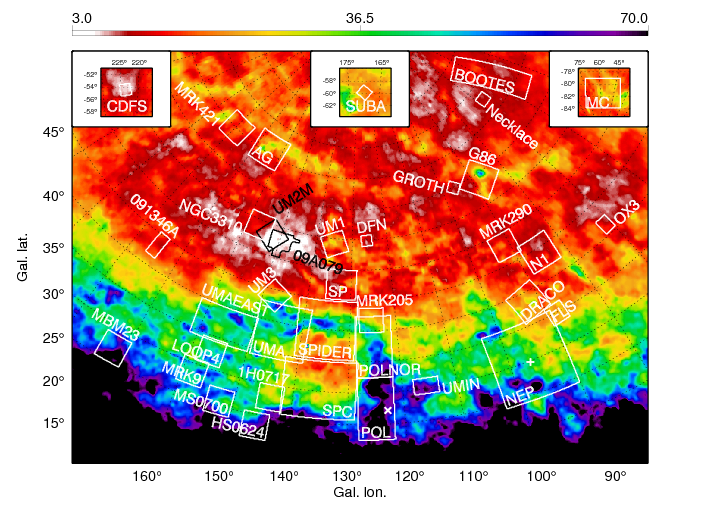
Fields whose names are italicized are embedded within a larger GHIGLS field. They are not shown in the figure nor are their details summarized in Martin et al. 2015. Data from H1821 are included in the NFD mosaic linked to below. Data for the remaining four are included within the NCPL mosaic.
Exploring and accessing the data
The GHIGLS data cubes can be explored by first clicking on the name of the field of interest, which opens a "data window" that provides further resources specific to the field.
Preview of the data cube
A preview movie is available at the top of the data window. The velocity extremes in the movie were selected to include all low, intermediate, and high velocity (LVC, IVC, and HVC) HI emission for the selected field. As in the colourbar in the locations figure, the brightest emission is blue. Each field has a scaling appropriate to the range of brightness temperature. A colourbar in K can be seen in the high-resolution movies described below.
Download the data cube
From the data window the original FITS data cube is available for download. This file has four extensions as follows:
- Ext[0] : Brightness temperature cube (K)
- Ext[1] : Mask map flagging those spectra where baselines were not removed
- Ext[2] : Noise map calculated from emission-free end channels (K)
- Ext[3] : Relative weight map output from AIPS sdgrd gridding routine
Movies
There are high-resolution movies in both MP4 and OGG formats. These can be viewed in a browser or downloaded.
Tumbling rendered cube
One way to visualize the spectral line cube is by rendering (see Fig. 2 in Martin et al. 2015). Changing the viewing angle can reinforce the sense of connectedness and separation of the structures, as illustrated in the tumbling cube movie: GHIGLS_[field name]_tumble.
Principal planes
Three are of the brightness temperature in sequences of planes perpendicular to the principal axes of the cube (see Fig. 3 in Martin et al. 2015).
- GHIGLS_[field name]: longitude-latitude channel maps on the sky, starting from the highest v.
- GHIGLS_[field name]_lv: longitude-velocity, viewed from the low-latitude face of the cube and starting at the lowest latitude.
- GHIGLS_[field name]_vb: velocity-latitude, viewed from the high-longitude face of the cube and starting at the highest longitude.
Mean, median, and standard deviation spectra
The overall velocity structure in the cube has been summarized on the data window. Mean (solid), median (dashed), and standard deviation (dotted) spectra are all shown (see Fig. 4 in Martin et al. 2015). The standard deviation spectrum has been used to identify HVC, IVC and LVC components (see next section).
Column density NHI
Also available for download on the data window is a FITS file containing maps of the integrated line emission, converted to column density NHI (using Ts = 80 K), for HVC, IVC, and LVC components whose velocity ranges are defined as in Planck Collaboration XXIV (2011) and Martin et al. (2015) using the shape of the standard deviation spectrum.
The column density maps are in units 1019 cm-2. The five planes in the NHI data cube correspond to HVC, IVC, LVC, IVC+LVC, and HVC+IVC+LVC.